
Introduction to Linear Algebra
Systems of Linear Equations
- Introduction
- Linear systems
- Vectors
- Linear combinations
- Matrices
- Planes in ℝ³
- Equation A x = b
- Sensitivity of solutions
- Linear independence
- Plane transformations
- Space transformations
- Linear transformations
- Affine maps
- Exercises
- Answers
Matrix Algebra
- Introduction
- Manipulation of matrices
- Partitioned matrices
- Block matrices
- Matrix operators
- Determinants
- Cofactors
- Cramer's rule
- Chiò's method
- Equivalent matrices
- Elimination: A = L U
- PLU factorization
- Reflection
- Givens rotation
- Special matrices
- Exercises
- Answers
Vector Spaces
- Introduction
- Motivation
- Vector spaces
- Bases
- Dimension
- Coordinate systems
- Linear transformations
- Change of basis
- Matrix transformations
- Compositions
- Isomorphisms
- Dual transformations
- Quotient spaces
- Wedge products
- Rotors
Eigenvalues, Eigenvectors
- Introduction
- Characteristic polynomials
- Companion matrix
- Algebraic and geometric multiplicities
- Minimal polynomials
- Eigenspaces
- Where are eigenvalues?
- Eigenvalues of A B and B A
- Generalized eigenvectors
- Similarity
- Diagonalizability
- Self-adjoint operators
- Exercises
- Answers
Euclidean Spaces
- Introduction
- Euclidean space
- Bilinear transformations
- Norm and distance
- Matrix norms
- Dual norms
- Dual transformations
- Examples of transformations
- Orthogonality
- Gram--Schmidt Process
- Orthogonal matrices
- Self-adjoint matrices
- Unitary matrices
- Projection operators
- QR-decomposition
- Least Square Approximation
- Quadratic forms
- Exercises
- Answers
Canonical forms
- Introduction
- 2D decomposition
- 3D decomposition
- Projectors
- Direct-sum decompositions
- Cyclic decompositions
- Symmetric matrices
- Symmetric matrices
- Pseudoinverse
- URV-decomposition
- LU-decomposition
- QR-decomposition
- Cholesky decomposition
- Schur decomposition
- Positive matrices
- Roots
- Polar factorization
- Spectral decomposition
- CUR decomposition
- Exercises
- Answers
Applications
- Introduction
- Circles along curves
- TNB frames
- GPS problem
- Coriolis acceleration
- Poisson equation
- Graph theory
- Error correcting codes
- Electric circuits
- FSA
- Markov chains
- Cryptography
- Wave-length transfer matrix
- Computer graphics
- Linear Programming
- Hill's determinant
- Fibonacci matrices
- Discrete dynamic systems
- Discrete Fourier transform
- Fast Fourier transform
- Curve fitting
- Answers
Miscellany
- Introduction
- Circles along curves
- TNB frames
- Differential forms
- Calculus
- Vector representations
- Matrix representations
- Change of basis
- Orthonormal Diagonalization
- Generalized inverse
- Differential forms
Preliminaries
- Complex Number Operations
- Sets
- Polynomials
- Polynomials and Matrices
- Computer solves Systems of Linear Equations
- Location of Eigenvalues
- Power Method
- Iterative Method
- Similarity and Diagonalization
Glossary
Reference

This Book is licensed under Creative Commons Attribution-NonCommercial-NoDerivs 3.0 Unported License
The Wolfram Mathematic notebook which contains the code that produces all the Mathematica output in this web page may be downloaded at this link. Caution: This notebook will evaluate, cell-by-cell, sequentially, from top to bottom. However, due to re-use of variable names in later evaluations, once subsequent code is evaluated prior code may not render properly. Returning to and re-evaluating the first Clear[ ] expression above the expression no longer working and evaluating from that point through to the expression solves this problem.
Remove[ "Global`*"] // Quiet (* remove all variables *)
Annihilators
Recall that V is an 𝔽-vector space over field 𝔽 (which is either ℚ or ℝ or ℂ). The set of all linear functionals is denoted by V✶ or V′ (the Riesz representation theorem establishes isomorphism between these two spaces, see Dual transformations in Part 5).From this definition, we immediately get that {0}0 = V* and V0 = {0}. If V is finite-dimensional and contains a non-zero vector, then Theorem 5 assures us that S0 ≠ V*.
- For any subset S of V, S0 = (span{S})0.
- For any subsets S₁ and S₂ of V, if S₁ ⊆ S₂, then S₂0 ⊆ S₁0.
- For any subset S of V, S0 is a subspace of V✶ and S ⊆ (S0)0.
-
Since S ⊆ span(S), we find that (span(S))0 ⊆ S0.
Conversely, suppose that φ ∈ S0, i.e., φ(s) = 0 for all s ∈ S. For any linear combination c1v1 + c2v2 + ⋯ + cnvn from span(S), where c1, c2, … , cn ∈ 𝔽 and v1, v2, … , vn ∈ S, we have \begin{align*} \varphi \left( c_1 {\bf v}_1 + c_2 {\bf v}_2 + \cdots + c_n {\bf v}_n \right) &= c_1 \varphi \left( {\bf v}_1 \right) + c_2 \varphi \left( {\bf v}_2 \right) + \cdots + c_n \varphi \left( {\bf v}_n \right) \\ &= 0 \end{align*} and hence φ ∈ (span(S))0.
- Suppose S₁ ⊆ S₂ and φ ∈ S₂. Then for any v ∈ S₁, φ(v) = 0 and consequently, φ ∈ S₁.
- Since for any v ∈ S, 0(v) = 0, we find that 0 ∈ S0, and therefore S0 ≠ ∅. Let φ, ψ ∈ S0 and c, k ∈ 𝔽. Then for every v ∈ S, \[ \left( c\varphi + k\psi \right) {\bf v} = c\varphi ({\bf v}) + k \psi ({\bf v}) = c0 + k0 \\ = 0 , \] which shows that S0 is subspace of V*. Now let v ∈ S. Then for every linear functional φ ∈ S0, v*(φ) = φ(v) = 0. So v* ∈ (S0)0; since V can be naturally identifies with V**, v ∈ (S0)0.
Let β = { x1, x2, … , xn } be a basis in V whose first m elements are in S (so they constitute a basis in S as being linearly independent). Let β* = { y1, y2, … , yn } be the dual basis in V*, We denote by R ⊂ V* the subspace spanned on { ym+1, ym+2, … , yn }. Clearly, R has dimension n−m. We are going to show that R = S0.
If x is any vector in S, then x is a linear combination of the first m elements from the basis β:
Let \( \displaystyle{\bf A} = \begin{bmatrix} a & b \\ c & d \end{bmatrix} , \) where 𝑎, b, c, and d are some real numbers to be determined. To find their values, we calculate A B − B A: \[ {\bf A}\,{\bf B} - {\bf B}\,{\bf A} = \begin{bmatrix} 2c - 2b & 3b + 2d - 2a \\ 2a - 3c - 2d & 2b - 2c \end{bmatrix} . \]
A = {{a, b}, {c, d}};
A.B - B.A
In order to determine W0, we use the dual basis {E1, E2, E3, E4} that corresponds to the standard basis of ℝ2,2: \[ {\bf E}_1 = \begin{bmatrix} 1 & 0 \\ 0 & 0 \end{bmatrix} , \quad {\bf E}_2 = \begin{bmatrix} 0 & 1 \\ 0 & 0 \end{bmatrix} , \quad {\bf E}_3 = \begin{bmatrix} 0 & 0 \\ 1 & 0 \end{bmatrix} , \quad {\bf E}_1 = \begin{bmatrix} 0 & 0 \\ 0 & 1 \end{bmatrix} . \] Arbitrary element from W0 can be expanded with respect to the dual basis \[ W^{0} \ni \varphi = c_1 {\bf E}^1 + c_2 {\bf E}^2 + c_3 {\bf E}^3 + c_4 {\bf E}^4 , \tag{14.2} \] where coefficients are determined from condition φ(A) = 0. Expansion of A with respect to standard basis is \[ {\bf A} = 2{\bf E}_2 + 2 {\bf E}_3 + 3 {\bf E}_4 . \] Then \[ W^{0} \ni \varphi ({\bf A}) = \left( c_1 {\bf E}^1 + c_2 {\bf E}^2 + c_3 {\bf E}^3 + c_4 {\bf E}^4 \right) \left( 2{\bf E}_2 + 2 {\bf E}_3 + 3 {\bf E}_4 \right) = {\bf 0} . \] Since action of elements from dual basis on standard basis elements are known, we get \[ W^{0} \ni \varphi ({\bf A}) = 2 c_2 + 2 c_3 + 3 c_4 = 0. \tag{14.3} \] Since there is one condition Eq.(14.3) between four coefficients in Eq.(14.2), we conclude that dimW0 = 3. ■
The second annihilator consists of all polynomials p such that φ(p) = p(0) = 0. A polynomial to be zero at the origin should be without a free term. Therefore, S00 = S.
Upon introducing a standard basis in ℝ≤n[x], \[ {\bf e}_0 =1, \ {\bf e}_1 = x, \ {\bf e}_2 = x^2 , \ \ldots , \ {\bf e}_n = x^n , \] we establish a one-to-one and onto (bijection) transofrmation f : ℝ≤n[x] ≌ ℝn+1 such that \[ f \left( a_0 + a_1 x + a_2 x^2 + \cdots + a_n x^n \right) = \left( a_0 , \ a_1 , \ a_2 , \ \ldots , \ a_n \right) . \] Then S is congruent to a subspace of ℝn+1: \[ S \cong \left\{ \left( 0 , x_1, x_2 , \ldots , x_n \right) \ : \ x_k \in \mathbb{R}, \quad k=1,2,\ldots , n \right\} . \]
Similarly, we can consider the subspace Sn of polynomials of degree at most n−1. Its annihilating functional acts as \[ \psi \left( a_0 , a_1 , a_2 , \ldots , a_{n-1} , a_n \right) = \left( a_0 , a_1 , a_2 , \ldots , a_{n-1} , 0 \right) \] In the space of polynomials ℝ≤n[x], this annihilating functional just drp the last term with xn. ■
Moreover, if κ is any functional over V and if v = x + y, we write x⁰(v) = κ(y) and y⁰(v) = κ(x). It is not hard to see that functions x⁰ and y⁰ thus defined are linear functionals on V, so x⁰ and y⁰ belong V*; they also belong to X⁰ and Y⁰, respectively. Since κ = x⁰ + y⁰, it follows that V* is indeed the direct sum of X⁰ and Y⁰.
To establish the asserted isomorphisms, we make a correspondence to every x⁰ a functional ψ from Y* defined by ψ(y) = x⁰(y). It can be shown that the correspondence x⁰ ↦ ψ is linear and one-to-one, and therefore an isomorphism between X⁰ and Y*. The corresponding result for Y⁰ and X* follows from symmetry by interchanging x and y.
Given vectors v and u are linearly independent because none is a scalar multiple of another. Therefore, W = span(v, u) is two-dimensional vector space.
We build an annihilator W0 using dual basis {e1, e2, e3, e4} to the standard basis e₁ = (1, 0, 0, 0), e₂ = (0, 1, 0, 0), e₃ = (0, 0, 1, 0), e₄ = (0, 0, 0, 1). Then any vector φ from W0 can be expressed as a linear combination of basis vectors: \[ \varphi = b_1 {\bf e}^1 + b_2 {\bf e}^2 + b_3 {\bf e}^3 + b_4 {\bf e}^4 , \] where scalars b₁, b₂, b₃, b₄ should be chosen so that φ(w) = 0 for any w ∈ W. So \[ W^{0} \ni \varphi ({\bf w}) = \left( b_1 {\bf e}^1 + b_2 {\bf e}^2 + b_3 {\bf e}^3 + b_4 {\bf e}^4 \right) \left( c_1 {\bf v} + c_2 {\bf u} \right) = 0 , \] where c₁, c₂ ∈ ℝ. Applying φ to basis vectors v and u, we get the system of equations: \begin{align*} \varphi ({\bf v}) &= \left( b_1 {\bf e}^1 + b_2 {\bf e}^2 + b_3 {\bf e}^3 + b_4 {\bf e}^4 \right) \left( 4, -3, 2, -1 \right) \\ &= 4\,b_1 -3\,b_2 + 2\, b_3 - b_1 = 0, \\ \varphi ({\bf u}) &= \left( b_1 {\bf e}^1 + b_2 {\bf e}^2 + b_3 {\bf e}^3 + b_4 {\bf e}^4 \right) \left( 1, 2, -1, 3 \right) \\ &= b_1 + 2 b_2 - b_3 + 3\,b_4 = 0 . \end{align*} Solving system of linear equations \[ \begin{split} 4\,b_1 -3\,b_2 + 2\, b_3 - b_1 &= 0, \\ b_1 + 2 b_2 - b_3 + 3\,b_4 &= 0 , \end{split} \]
Now, on the other hand, suppose that ϕ ∈ (S⁰ ∩ T⁰). Then ϕ annihilates both S and T. If v ∈ S + T, then v = s + t, where s ∈ S and t ∈ T. Now ϕ(v) = ϕ(s + t) = ϕ(s) + ϕ(t) = 0 + 0 = 0. This shows that ϕ annihilates S + T, i.e., ϕ ∈ (S + T)⁰. Therefore, (S⁰ ∩ T⁰) ⊆ (S + T)⁰ and hence (S⁰ ∩ T⁰) = (S + T)⁰.
Also, if φ = ψ + χ ∈ S⁰ + T⁰, where ψ ∈ S⁰ and χ ∈ T⁰, then ψ, χ ∈ (S ∩ T)⁰, and so φ ∈ (S ∩ T)⁰. Thus, \[ S^0 + T^0 \subseteq \left( S \cap T \right)^0 . \] For the reverse inclusion, suppose that φ ∈ ( S ∩ T)⁰. Write \[ V = S' \oplus \left( S \cap T \right) \oplus T' \oplus U , \] where S = S' ⊕ (S ∩ T) and T = T' ⊕ (S ∩ T). Define χ ∈ V* by \[ \left. \chi \right\vert_{S'} = \phi , \qquad \left. \chi \right\vert_{S \cap T} = \left. \phi \right\vert_{S \cap T} = 0 , \qquad \left. \chi \right\vert_{T'} = 0 , \qquad \left. \psi \right\vert_{U} = \phi , \] and define ψ ∈ V* by \[ \left. \psi \right\vert_{S'} = 0 , \qquad \left. \psi \right\vert_{S \cap T} = \left. \phi \right\vert_{S \cap T} = 0 , \qquad \left. \psi \right\vert_{T'} = \phi , \qquad \left. \psi \right\vert_{U} = 0 . \] It follows that &χ ∈ T⁰, ψ ∈ S⁰ and χ + ψ = φ.
We can also derive the second partof this statement from the first part by replacing S by S⁰ and T by T⁰, and using the identity S⁰⁰ = S, we get (S⁰ + S⁰)⁰ = (S⁰)⁰ ∩ (T⁰)⁰ = S ∩ T.
Hyperplanes/Hyperspaces
With dot-product, we can make the following (geometric) definition.
A linear equation a • x = b is a constraint on our choice of a point in 𝔽n. With such constraint, we expect to lose a degree of freedom on the solution set for the linear equation. When choosing a point x = (x₁, x₂, … , xn) in 𝔽n, we have n degrees of freedom---the number of coordinates. By satisfying a single linear equation, we expect to have n − 1 degrees of freedom.
In case of general finite dimensional vector space V, a maximal proper subspace of V is called a hyperspace of V. A hyperplane is a coset of a hyperspace.

According to the rank nullity theorem. the dimension of the domain of a linear transformation φ is the sum of the rank of φ (the dimension of the image of φ) and the nullity of φ (the dimension of the kernel of φ). Since the dimension of the image of φ is 1 (it is either ℝ or ℂ---both are one dimensional spaces), we conclude that the kernel (null space) of φ has dimension n−1, so it is hyperspace.
Conversely, suppose that W is a hyperspace of V. Then we have to construct a nonzero linear functional ψ on V such that null space of ψ is W, as {0} ≠ W ≠ V. There exists a basis u1, u2, … , un-1 ∈ W because the dimension of a hyperspace is 1 less than dimension of V. Let 0 ≠ u be a vector in V that does not belong to W. If we set ψ(u) = 1, but ψ annihilates every element from the basis uj (j = 1, 2, … , n−1), then ψ becomes the required linear form.
n = Graphics[{Blue, Thickness[0.01], Arrowheads[0.1], Arrow[{{0, 0}, {-0.5, 1}}]}];
ver = Graphics[{Dashed, Line[{{0, -0.5}, {0, 1}}]}];
txt1 = Graphics[ Text[Style["2 x + y = 0", 25, Italic, Black], {0.5, 0.5}]];
txt2 = Graphics[Text[Style["n", 25, Bold, Black], {-0.25, 0.95}]];
Show[hor, ver, n, line, txt1, txt2]
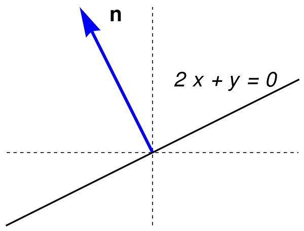
This is a wonderful benefit of numeric/geometric duality: if we have a homogeneous linear equation in two variables, we can visualize its solution as a line.
We can do the same job algebraically too. If we solve 2 x + y = 0 by row- reducing the one-rowed matrix [2 1] ∼ [1, 1/2], we get one free column, and hence one homogeneous generator h = [−1, 2]. Our solution mapping consequently takes the form \[ H(t) = t\,{\bf h} = t\left[ -2, \ 1 \right] . \]
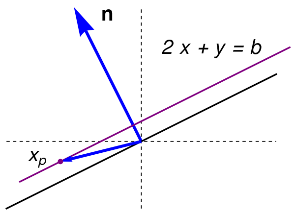
Now consider an inhomogeneous two-variable equation \[ {\bf a} \bullet {\bf x} = b \qquad (b \ne 0) . \tag{18.2} \] Solve this by row-reducing the one-rowed augmented matrix \[ \left[ 2 \ 1 \vert \ b \right] . \] In our example, a = [2, 1] ≠ (0, 0), so we must get a pivot when we row-reduce. That leaves one free column, producing one homogeneous generator h that we found previously. The general solution of the inhomogeneous equation a • x = b therefore takes the form \[ {\bf x}(t) = {\bf x}_p + {\bf x}_h = {\bf x}_p + t\,{\bf h} , \] where xp is a particular solution of the nonhomogeneous equation (18.2) and xh is the general solution of the corresponding homogeneous equation. Here h = [−1, 2] is the homogeneous generator for the sequation (18.1).
line2 = Graphics[{Purple, Thick, Line[{{-0.9, -0.3}, {1.1, 0.7}}]}];
n = Graphics[{Blue, Thickness[0.01], Arrowheads[0.1], Arrow[{{0, 0}, {-0.5, 1}}]}];
ver = Graphics[{Dashed, Line[{{0, -0.5}, {0, 1}}]}];
arr = Graphics[{Blue, Thickness[0.01], , Arrowheads[0.04], Arrow[{{0.0, 0}, {-0.6, -0.15}}]}];
txt1 = Graphics[ Text[Style["2 x + y = b", 25, Italic, Black], {0.5, 0.77}]];
txt2 = Graphics[Text[Style["n", 25, Bold, Black], {-0.25, 0.95}]];
xp = Graphics[ Text[Style[Subscript[x, p], 25, Italic, Black], {-0.77, -0.1}]];
disk = Graphics[{Purple, Disk[{-0.6, -0.15}, 0.02]}];
Show[hor, ver, n, line, line2,arr,txt1, txt2,xp,disk]
Using isomorphisms of vector spaces ℝn ≌ ℝ1×n ≌ ℝn×1, we rewrite the homogeneous equation in matrix/vector form
- Axler, Sheldon Jay (2015). Linear Algebra Done Right (3rd ed.). Springer. ISBN 978-3-319-11079-0.
- Halmos, Paul Richard (1974) [1958]. Finite-Dimensional Vector Spaces (2nd ed.). Springer. ISBN 0-387-90093-4.
- Katznelson, Yitzhak; Katznelson, Yonatan R. (2008). A (Terse) Introduction to Linear Algebra. American Mathematical Society. ISBN 978-0-8218-4419-9.
- Treil, S., Linear Algebra Done Wrong.
- Wikipedia, Dual space/