In this section you learn a
remarkable result
that for linear operators on a finite-dimensional vector space, either injectivity or
surjectivity alone implies the other condition. Often it is easier to check that
an operator on a finite-dimensional vector space is injective, and then we get
surjectivity for free.
Inverse Matrices I
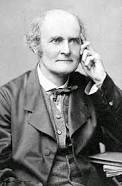
Arthur Cayley
Suppose that A is a square matrix. We want to find a matrix (which we denote naturally by A-1)
of the same size, such that A-1timesAequalsI, the identity matrix.
Whatever A does or transforms to, A-1 undoes or transforms back. Their product is the
identity matrix, which does nothing. The problem is that such inverse matrix might not exist. The notion of the
inverse of a matrix first appears in an 1855 note of Arthur Cayley (1821--1895). In 1842, Arthur Cayley graduated from
Trinity College, Cambridge, England, but could not find a suitable teaching post. So for 14 years starting 1863,
he worked as a lawyer. During this time frame, he published about 300 mathematical papers, and finally, in 1863, he
became a professor at Cambridge.
A square n × n matrix A is invertible or not singular if there exists a matrix A-1
such that
where I = In is the identity matrix of size n.
Apparently, a square matrix for which does not exist an inverse matrix is called singular. The set of n×n invertible matrices over field 𝔽 is called the general linear group of degree n, which is denoted by GL(n, 𝔽) or GLn(𝔽), or simply GL(n) if the field is understood.
Non-square matrices (m-by-n matrices for which m ≠ n) do
not have an inverse. However, in some cases such a matrix may have a
left inverse or right inverse.
If m-by-n matrix A is tall (m ≥ n) and its rank is equal to n, then
A has a left inverse: an n-by-m matrix P such that
P A = In.
If m-by-n matrix A is wide (n ≥ m) and its rank is m, then it has a
right inverse: an n-by-m matrix Q such that
A Q = Im.
There are known many other generalized inverses.
In other sections, we will work with the pseudoinverse, which is sometimes called the
Moore–Penrose inverse, when we discuss
least squares approximations and singular value decomposition. However, there are known others such as
group inverse and Drazin inverse.
Raymond Beauregard
Theorem: (Raymond Beauregard)
For any n × n matrices A and C over a field of
scalars 𝔽,
Recall that if A is n × n matrix then its reduced row-echelon form
H is a
matrix of the same size with zeros in the pivot columns except for the pivots
which are equal to 1. It is achieved by applying elementary row operations
(row swapping, row addition, row scaling) to A. An elementary matrix is
one obtained by applying a single elementary row operation to the n × n
identity matrix I. Elementary matrices have inverses that are also
elementary matrices. Left multiplication of A by an elementary matrix
E effects the same row operation on A that was used to create
E. If P is a product of those elementary matrices that reduce
A to P, then P is invertible and PA =
H.
Let H be the reduced row echelon form of A, and let P be
the product of those elementary matrices (in the appropriate order) that
reduce A to H. P is an invertible matrix such that
P A = H. Notice that H is the identity matrix if and only
if it has n pivots.
Beginning with A C = I, we left multiply this equation by P
obtaining \( {\bf P}\,{\bf A}\,{\bf C} = {\bf P} \)
or \( {\bf H}\,{\bf C} = {\bf P} . \) If H
is not the identity matrix it must have a bottom row of zeros forcing P
to have likewise a bottom row of zeros, and this contradicts the
invertibility of P. Thus H = I, C = P, and
the equation \( {\bf P}\,{\bf A} = {\bf H} \) is
actually \( {\bf C}\,{\bf A} = {\bf I} . \)
This argument shows at once that (i) a matrix is invertible if and only if its
reduced row echelon form is the identity matrix, and (ii) the set of
invertible matrices is precisely the set of products of elementary matrices.
From Beauregard's theorem, it follows that the inverse matrix is unique. Although, we can show directly that a matrix
A cannot have two different inverses. Suppose the opposite is true and there exist two matrices B and
C such that BA = I and AC = I. According to the identities
Corollary 1:
If B is left inverse of A and C is right inverse of A, then B = C.
Suppose that A C = B A = I, the identity matrix. Then
\[
{\bf C} = {\bf I}\,{\bf C} = \left( {\bf B}\,{\bf A} \right) {\bf C} = {\bf B} \left( {\bf A}\,{\bf C} \right) = {\bf B}\,{\bf I} = {\bf B} .
\]
Note that not every square matrix has an inverse matrix. For example, matrix
\( \displaystyle \begin{bmatrix} 1& 2 \\ 1&2 \end{bmatrix} \) has no inverse because it does not satisfy conditions of Theorem 10.
Theorem 5:
Let A and B be two matrices of the same dimension.
If A B is invertible, then each of A and B is invertible.
The shortest proof follows from the formula for determinants:
\[
\det \left({\bf A}\,{\bf B} \right) = \det\left( {\bf A} \right) \det\left( {\bf B} \right) .
\]
To prove the theorem 5, we consider matrices as operators that generate linear transformations. So every m × n matrix A corresponds a linear transformation TA : 𝔽n ⇾ 𝔽m. Therefore, we reformulate this theorem in terms of transformations:
Let T : 𝔽n ⇾ 𝔽n and S : 𝔽n ⇾ 𝔽n be linear transformation so that their composition T∘S : 𝔽n ⇾ 𝔽n is also a linear transformation. If T∘S is an isomorphism, then both S and T are isomorphisms.
Since T S = T∘S is an isomorphism, it is both 1-1 (injective) and onto (surjective). Then S is 1-1, for if
there were some nonzero vector u ∈ 𝔽n with
S(u) = 0, then we would have T S(u) = T(0) = 0 and T would not be injective. Also, T is onto, for if there were some vector w with w ≠ T(v) for any v in 𝔽n, then certainly w ≠ T S(u) for any u ∈ 𝔽n.
Another proof:
Since the product of two matrices A B is invertible, then there exists a right inverse
\[
{\bf A}\,{\bf B}\,{\bf R} = {\bf I} \qquad \Longrightarrow \qquad {\bf A} \left( {\bf B}\,{\bf R} \right) = {\bf I} .
\]
So the product B R is a right inverse of A. From Beauregard's theorem, we conclude that A is invertible.
Since A is invertible, multiplying by A−1, we get B = A−1P for some invertible matrix P. This shows that B is a product of two invertible matrices; hence, it is also inverticle.
Example 4:
Let
\[
{\bf A} = \begin{bmatrix} 2& -1& 3 \\ 1& -3& 2 \\ 3& -2& 4 \end{bmatrix} , \qquad {\bf B} = \begin{bmatrix} 5& 3& -4 \\ 5& 2& -4 \\ 3& 5& -2 \end{bmatrix} .
\]
Their product
\[
{\bf A}\,{\bf B} = \begin{bmatrix} 14& 19& -10 \\ -4& 7& 4 \\ 17& 25& -12 \end{bmatrix}
\]
is not singular because its row reduce echelon form is the identity matrix.
Clear[A, B, t, x, P];
A = {{2, -1, 3}, {1, -3, 2}, {3, -2, 4}};
B = {{5, 3, -4}, {5, 2, -4}, {3, 5, -2}};
AB = A . B
But when tried to determine the inverse of B, Mathematica disagrees with us:
Inverse[B]
Inverse: Matrix B is singular
Similar outcomes we obtain for their products,
Inverse[AB]
Inverse: Matrix AB is singular
Inverse[BA]
Inverse: Matrix BA is singular
This example shows that a product of two matrices is a singular matrix when one of the multiples is not invertible.
End of Example 5
This theorem confirms the common sense: If one put on socks and then sneakers, the first to be taken off are sneakers.
Given A ∈ 𝔽m×n, the transpose of A = [ai,j], denoted
AT ∈ 𝔽n×m or just A', is a matrix
defined by \( \left[ a_{i,j}
\right]^{\mathrm T} = \left[ a_{j,i} \right] . \)
Theorem 7: Let A be a rectangular m × n matrix with real entries. Then the product ATA
is an invertible n × n matrix if and only if
A has linearly independent columns (full column rank). This statement is valid for complex-valued matrices,
but instead of ATA it should be considered A*A, the product of the adjoint matrix (conjugate transpose) with itself.
The product is a square matrix (n-by-n). For every matrix A, we are going to show that ATA
has the same kernel as A. When the columns of
A are linearly independent, its nullspace contains only the zero vector. Then ATA
with this same nullspace, is invertible.
Let A be any matrix. If vector x is in its kernel, then Ax = 0. Multiplying by AT
gives
\( {\bf A}^{\mathrm T}{\bf A} \,{\bf x} = {\bf 0} . \) So x is also in the
nullspace of ATA.
Now start with the kernel of \( {\bf A}^{\mathrm T}{\bf A} . \) From
\( {\bf A}^{\mathrm T}{\bf A} \,{\bf x} = {\bf 0} , \) we must prove that
Ax = 0. We multiply from left by \( {\bf x}^{\mathrm T}: \)
The vector \( {\bf A} \,{\bf x} \) has length zero. Therefore,
\( {\bf A} \,{\bf x} = {\bf 0} . \) Every vector x in one nullspace is in the other nullspace.
If A is of full column rank, so does ATA.
If A has independent columns, so does
\( {\bf A}^{\mathrm T}{\bf A} . \)
Example 6:
We consider a complex 3 × 3 matrix
\[
{\bf A} = \begin{bmatrix} 3& {\bf j}& -1 \\ 1 + {\bf j}& 4& -3 + 3 {\bf j} \\ 1& 3& -2 + {\bf j} \end{bmatrix} .
\]
This is the time to mention that a conflict exists over the proper notation for the imaginary unit number. Some (mostly physicists, engineers, and computer scientists) contend the symbol ⅉ, which should be \[ImaginaryJ] in Wolfram language; others (mostly mathematicians and economists) believe it should be ⅈ, with code \[ImaginaryI] or just I. This unresolved conflict creates confusion. As the Wolfram language was written mostly by mathematicians (despite Stephen Wolfram having been a Physics major), Mathematica resolves the conflict by outputting the \[ImaginaryJ] as I, note below. Also, some texts use a wrong notation for this symbol as \( \displaystyle \sqrt{-1} \) because a square root is not a function and a square root assigns two outputs for each input. So the correct notation should be as follows: \( \displaystyle \sqrt{-1} = \pm ⅉ . \)
Using Mathematica, it is easy to check that matrix A is not singular; just check its determinant to be nonzero:
In mathematics and engineering, it is common to denote by i, j, and k unit vectors in a three dimensional space. Since on complex plane ℂ, the imaginary unit is in positive vertical direction and coinsides with j, it is natural to denote it as ⅉ; however, since vectors in this tutorial are denoted with lower case letters in bold font, we alsways utilize j for the imaginary unit.
Portions of this website are created in HTML code that is agnostic about notation formalities in mathematics. Below, the j is used for the imaginary unit number. This back-and-forth, frustrating as it is and may seem, is common in the field. The reader is encouraged to transform the field or become flexible in his thinking on this matter. The latter will take less time.
Its adjoint (which is complex conjugate and transposed) is
\[
{\bf A}^{\ast} = \left( \overline{\bf A} \right)^{\mathrm T} = \begin{bmatrix} 3&1-{\bf j}&1 \\ -{\bf j}& 4&3 \\ -1&-3-3{\bf j} & -2-{\bf j} \end{bmatrix} .
\]
We use notation \( \displaystyle \overline{\bf A} \) for complex conjugate, as it is common in mathematics. However, in physics, compelx conjugate operation is denoted by asterisk (which we reserve for adjoint). As you see, my intention to please everyone leads to confusion---I am not responsible for it!
aA = ConjugateTranspose[A]
{{3, 1 - I, 1}, {-I, 4, 3}, {-1, -3 - 3 I, -2 - I}}
{{11, 6 + 4 I, 5 + 4 I}, {6 - 4 I, 36, 22 - 2 I}, {5 - 4 I, 22 + 2 I,
15}}
aAA = aA.A
{{12, 7 - I, -5 + 7 I}, {7 + I,
26, -18 + 16 I}, {-5 - 7 I, -18 - 16 I, 24}}
The notation problem re-appears in the superscripts denoting the adjoint matrix. In Mathematica A* is the Conjugate and A\[ConjugateTranspose] is the ConjugateTranspose. Above the HTML uses the asterisk (*) for the adjoint matrix. Below Mathematica uses the dagger (\[ConjugateTranspose]). Deal with it.
TrueQ[SuperStar[A] = A\[Conjugate]]
False
Note that Mathematica tells us that statement is not true. Make a very close inspection of the character to the right of A and you will see they are not the same. The left hand side is A with a superscript asterisk; the right hand side is A with a special character entered (esc)co(esc) of (esc)conj(esc) which is shorthand for the conjugate. The Wolfram documentation clarifies.
Example 7:
Let us consider the diagonal matrix
\[
\Lambda = \begin{bmatrix} 2&0&0&0 \\ 0&-3&0&0 \\ 0&0&4&0 \\ 0&0&0&-9 \end{bmatrix} .
\]
Although this matrix is equivalent to a vector u = [2, −3, 4, −9], the advantage of the matrix representation is that we can define its inverse, which is not permitted for vectors. So we have
\[
\Lambda^{-1} = \begin{bmatrix} \frac{1}{2}&0&0&0 \\ 0&-\frac{1}{3}&0&0 \\ 0&0&\frac{1}{4}&0 \\ 0&0&0&-\frac{1}{9} \end{bmatrix} .
\]
End of Example 7
Theorem 8: Equivalent Statements regarding a square n × n matrix A. The following statements are equivalent. That is, for a given matrix A, the statements are either all true or all false.
A is invertible.
The linear transformation TA : 𝔽n ⇾ 𝔽n generated by matrix A is an isomorphism.
There exists a left inverse matrix L such that L A = In, the identity matrix.
There exists a right inverse matrixR such that A R = In, the identity matrix.
A is row equivalent to the identity matrix In, so rref(A) = In.
The equation A x = 0 has only the trivial (= zero) solution.
A is expressible as a product of elementary matrices.
The equation A x = b has a unique solution for each n-component column vector b (which is an n × 1 matrix).
For any b ∈ 𝔽n×1, the equation A x = b has a solution.
The span (= set of all linear combinations) of the column vectors of A is 𝔽n×1.
detA ≠ 0.
The spectrum (= set of all eigenvalues) of matrix A does not contain zero.
\( \left( {\bf A}^{-1} \right)^{\ast} = \left( {\bf A}^{\ast} \right)^{-1} \qquad
\Longrightarrow \qquad \left( {\bf A}^{-1} \right)^{\mathrm T} = \left( {\bf A}^{\mathrm T} \right)^{-1} . \)
This means that A is invertible if and only if its adjoint (or conjugate transpose) matrix is invertible.
This theorem does not include all possible conditions of invertibility of matrices. For example, condition (b) on transformation TA to be isomorphism is too general. Indeed, it is sufficient to assume this transformation to be either surjective or injective aimilar to conditions (c) and (d) of a square matrix to have either left inverse or right inverse.
(a) ⇒ (b) Suppose that (a) is true. Then mapping TA is invertible, i.e., TA has an inverse transformation. Then
\begin{align*}
T_A T_A^{-1} &= T_A^{-1} T = I, \\
\left( T_A \right) \left( T_A \right)^{-1} &= \left( T_A \right)^{-1}T_A = I, \\
T_{A} T_{A^{-1}} &= T_{A^{-1}} T_{A} = I .
\end{align*}
So (b) is true.
(b) ⇒ (a) Since the chain equations in the previous part is reversible, so if (b) is true, then (a) is also true.
(a) ⇔ (h) Now recall that TA is the linear transformation. We know
that TA is invertible, i.e., TA is an isomorphism, if and only if TA is 1-1 and onto, i.e.,
if TA(x) = b has a unique solution for every b. Hence,
so (h) is equivalent to (a).
(a) ⇔ (i) Now the condition that TA is onto is the condition that TA(x) = b has a solution for every b, i.e., that A x = b has a solution for every b. This is just condition (i).
(a) ⇔ (d) The existence of a right inverse to A is equivalent that the corresponding transformation TA is onto.
(a) ⇔ (c) The existence of a left inverse to A is equivalent that the corresponding transformation TA is injective, which indeed is isomorphism.
(a) ⇔ (i) If A is invertible then x = A−1b is a solution of the linear system A x = b, since
\[
{\bf A} \left( {\bf A}^{-1} {\bf b} \right) = \left( {\bf A}\,{\bf A}^{-1} \right) {\bf b} = {\bf I}\,{\bf b} = {\bf b} .
\]
(i) ⇔ (h) To see that this solution is unique, suppose that there were two solutions
x, y ∈ 𝔽n×1. Then A x = b and A y = b, so subtracting gives us A(x − y) = 0. It then follows that
\begin{align*}
{\bf x} - {\bf y} &= \left( {\bf A}^{-1} {\bf A} \right) \left( {\bf x} - {\bf y} \right) = {\bf A}^{-1} \left( {\bf A} \left( {\bf x} - {\bf y} \right) \right) = {\bf A}^{-1} \left( {\bf A} \,{\bf x} - {\bf A} \,{\bf y} \right)
\\
&= {\bf A}^{-1} \left( {\bf b} - {\bf b} \right) = {\bf A}^{-1} {\bf 0} = {\bf 0} .
\end{align*}
So x = y and solution to A x = b is unique.
(h) ⇔ (f) It follows simply by choosing b = 0.
(h) ⇔ (e) If we represent the linear system A x = 0 in augmented matrix form [A | 0] and then apply Gauss–Jordan elimination, we get the augmented matrix [R | 0], where R is the reduced row echelon form of A. Since R is square, if R ≠ I, then it must have a row of zeros at the bottom,
so this linear system must have at least one free variable and thus cannot have
a unique solution. We thus conclude that if the linear system A x = 0 does have a unique solution (i.e., (f) holds) then R = I (i.e., (e) holds).
(e) ⇔ (g) If the RREF of A is I, then there exists a sequence of row operations that transforms A into I. Equivalently, there exists a finite sequence of elementary matrices E₁, E₂, … , Es such that Es ⋯ E₂ E₁ A = I. By
multiplying on the left by \( \displaystyle {\bf E}_s^{-1} {\bf E}_{s-1}^{-1} \cdots {\bf E}_1^{-1} , \) we see that
\[
{\bf A} = {\bf E}_1^{-1} {\bf E}_2^{-1} \cdots {\bf E}_s^{-1} .
\]
Since the inverse of an elementary matrix is again an elementary matrix, A can be written as a product of elementary matrices, so (f) follows.
(g) ⇔ (a) It follows from the facts that elementary matrices are invertible, and the product of invertible matrices is invertible.
(h) ⇔ (i) It is trivial.
(i) ⇔ (e) If we choose b ∈ 𝔽n×1 so that applying Gauss–Jordan elimination to the augmented matrix
[A | b] produces [R | en], where R is the reduced row echelon form of A. If R
had a zero row at the bottom, then this linear system would not have a solution.
However, since we are assuming (i) holds, this cannot be the case. It follows
that R must have no zero rows, so it equals I, which completes the
proof.
(a) ⇔ (k) Let R be the reduced row echelon form of A, which we abbreviate as rref(A). As a preliminary step, we will show that det(A) and det(R) are both zero or both nonzero. Let E₁, E₂, … , Es be the elementary matrices that correspond to the elementary row operations that produce R from A. Thus,
\[
{\bf R} = {\bf E}_s {\bf E}_{s-1} \cdots {\bf E}_1 {\bf A} .
\]
Since a determinant of a product of matrices is equal to the product of determinants, we get
\[
\det\left( {\bf R} \right) = \det\left( {\bf E}_s \right) \cdot \det\left( {\bf E}_{s-1} \right) \cdots \det\left( {\bf E}_1 \right) \cdot \det\left( {\bf A} \right) .
\]
We note that every elementary matrix has a nonzero determinant. Therefore, det(A) and det(R) are either both zero or both nonzero. If we assume that A is invertible, then it follows from (g) that R = I and hence that det(R) = det(I) = 1 ≠ 0. Thus, in turn, it implies that det(A) ≠ 0, which is what we want.
Conversely, assume that det(A) ≠ 0. It follows that det(R) ≠ 0. which tells us that R cannot have a row of zeroes. Thus, it follows that R = I, so A is invertible.
(c) ⇔ (k) Given L A = In, take determinants and use the product formula to get
det(L) det(A) = det(In) = 1𝔽. Since 1𝔽 ≠ 0𝔽 in a field 𝔽, this forces det(A) ≠ 0𝔽.
Example 8:
We break this example into multiple parts.
Example 8b:(b) Any isomorphism is characterized by existence of the inverse transformation, which in our case is known explicitly: \( \displaystyle T_A^{-1} = T_{A^{-1}} .eg\)
Example 8cd:(c) + (d)
Since a nonsigular matrix has an inverse, this inverse matrix is simulteneously left and right inverse.
Example 8eg:(e) + (g)
We consider the matrix
\[
{\bf A} = \begin{bmatrix} 1& 2& -2 \\ 3& 1& -2 \\ 3& 2& -3 \end{bmatrix} .
\]
The corresponding augmented matrix for inverse matrix determinantion is
aug = ArrayFlatten[{{A, IdentityMatrix[3]}}]
\[
\left[{\bf A}\mid{\bf I}\right] = \begin{bmatrix} 1& 2& -2 &1&0&0 \\ 3& 1& -2 &0&1&0 \\ 3& 2& -3 &0&0&1 \end{bmatrix} .
\]
We apply row reduction and write a corresponding elementary matrix. As first two steps, we eliminate both "3" in the first column by adding (−3)*first row. We abbreviate it as R2 ← (−3)·R1 + R2 and R3 → (−3)·R1 + R3
\[
\left[{\bf A}\mid{\bf I}\right] \,\underset{R}{\sim}\, \left[ \begin{array}{ccc|ccc} 1& \phantom{-}2& -2 &\phantom{-}1&0&0 \\ 0& -5& \phantom{-}4 &-3&1&0 \\ 0& -4& \phantom{-}3 &-3&0&1 \end{array} \right] , \qquad {\bf E}_1 = \begin{bmatrix} \phantom{-}1&0&0 \\ -3&1&0 \\ -3&0&1 \end{bmatrix} .
\]
Example 8hi:(h) + (i) We consider matrix/vector equation A x = b, where
\[
{\bf A} = \begin{bmatrix} 1& 2& -2 \\ 3& 1& -2 \\ 3& 2& -3 \end{bmatrix} ,
\]
and b is an arbitrary vector from ℝ3×1. Since matrix A is invertible, the given system of equations has an explicit solution
\[
{\bf x} = {\bf A}^{-1} {\bf b} , \qquad {\bf A}^{-1} = \begin{bmatrix} 1& 2& -2 \\ 3& 3& -4 \\ 3& 4& -5 \end{bmatrix} .
\]
Example 8m:(m) We consider the following complex valued matrix
\[
{\bf A} = \begin{bmatrix} 1& {\bf j}& 3 \\ 1 + {\bf j}&
2\,{\bf j}& -{\bf j} \\ 2 + {\bf j}& 2 - {\bf j}& 3 - {\bf j} \end{bmatrix} ,
\]
where j is the imaginary unit on the complex plain ℂ, with j² = −1. Its determinant and inverse can be found with the aid of Mathematica:
Again, despite being entered as imaginary j (\[ImaginaryJ] or ⅉ), Mathematica converts it to imaginary unit i (I or ⅈ) in the output. The reader is encouraged to research the tension between mathematicians and physicists and economists over the matter of the proper notation for the imaginary unit number.
Clear[A, B, t, x, P, S];
Inverse[A]*250
{{17 + 94 I, 67 - 56 I, 23 - 64 I}, {-25 - 50 I, -25 - 50 I,
25 + 50 I}, {61 - 23 I, -39 + 27 I, 9 + 13 I}}
Note that one half of the absolute value squared of the Determinant of A is a constant = 250 because 22² + 4² = 500.
\[
{\bf A}^{-1} = \frac{1}{\det({\bf A})} \begin{bmatrix} 17 + 94 {\bf j}& 67 - 56 {\bf j}& 23 - 64 {\bf j} \\ -25 - 50 {\bf j}& -25 - 50 {\bf j}&
25 + 50 {\bf j} \\ 61 - 23 {\bf j}& -39 + 27 {\bf j}& 9 + 13 {\bf j} \end{bmatrix} , \qquad \det({\bf A}) = 22 - 4{\bf j} .
\]
The adjoint of the inverse matrix in provided by Mathematica again
ConjugateTranspose[%]
{{17 - 94 I, -25 + 50 I,
61 + 23 I}, {67 + 56 I, -25 + 50 I, -39 - 27 I}, {23 + 64 I,
25 - 50 I, 9 - 13 I}}
Note that all coefficients of the Inverse of A are either 250 or one half of 250.
\[
\left( {\bf A}^{-1} \right)^{\ast} = \frac{1}{250} \begin{bmatrix} 17 - 94 {\bf j}& -25 + 50 {\bf j}&
61 + 23 {\bf j}& \\ 67 + 56 {\bf j}& -25 + 50 {\bf j}& -39 - 27 {\bf j} \\ 23 + 64 {\bf j}& 25 - 50 {\bf j}& 9 - 13 {\bf j} \end{bmatrix} .
\]
Now we consider the adjoint matrix (which is complex conjugate of transposed matrix)
At = ConjugateTranspose[A]
{{1, 1 - I, 2 - I}, {-I, -2 I, 2 + I}, {3, I, 3 + I}}
(b) Since A−1A = I, it follows that det(A−1A) = det(I) = 1. Therefore, we must have det(A−1A) = det(A−1) det(A) = 1. Since det(A) ≠ 0, the proof can be completed by dividing through by det(A).
(c) To see why part (c) holds, we just compute the product of kA and its
proposed inverse in both ways:
\[
\left( k\,{\bf A} \right) \left( \frac{1}{k}\,{\bf A}^{-1} \right) = \frac{k}{k}\,{\bf A}\,{\bf A}^{-1} = {\bf I} ,
\]
and
\[
\left( \frac{1}{k}\,{\bf A}^{-1} \right) \left( k\,{\bf A} \right) =
\frac{k}{k}\,{\bf A}^{-1}{\bf A} = {\bf I} .
\]
(d)
(e)
(f) Since we are given a formula for the proposed inverse, we just need to verify it by
multiplying it by A B and see that we do indeed get the identity matrix:
\[
\left( {\bf A}\,{\bf B} \right) \left( {\bf B}^{-1} {\bf A}^{-1}\right) = {\bf A} \left( {\bf B}\,{\bf B}^{-1} \right) {\bf A}^{-1} = {\bf A}\,{\bf I}\, {\bf A}^{-1} = {\bf I}
\]
and
\[
\left( {\bf B}^{-1} {\bf A}^{-1} \right) \left( {\bf A}\,{\bf B} \right) = {\bf B}^{-1} \left( {\bf A}^{-1} {\bf A} \right) {\bf B} = {\bf B}^{-1}{\bf I}\, {\bf B} = {\bf I} .
\]
Since both products result in the identity matrix, we conclude that A B is indeed
invertible, and its inverse is B−1A−1, as claimed.
Example 9:
Example 9a:(a) The inverse of the 3-by-3 matrix is
\[
{\bf A} = \begin{bmatrix} 1& 2& -2 \\ 3& 1& -2 \\ 3& 2& -3 \end{bmatrix} , \qquad {\bf A}^{-1} = \begin{bmatrix} 1& 2& -2 \\ 3& 3& -4 \\ 3& 4& -5 \end{bmatrix} .
\]
A = {{1, 2, -2}, {3, 1, -2}, {3, 2, -3}};
Ai = Inverse[A]
{{1, 2, -2}, {3, 3, -4}, {3, 4, -5}}
Then the double inverse is
\[
\left( {\bf A}^{-1} \right)^{-1} = {\bf A} .
\]
Inverse[Inverse[A]] == A
True
Example 9b:(b) We consider a 3 × 3 matrix
\[
{\bf A} = \begin{bmatrix} 3& 1& 1 \\ 9& 2& 2 \\ 7& 2& 3 \end{bmatrix} .
\]
Its determinant is
\[
{\bf A}^{-1} = \frac{1}{3} \begin{bmatrix} -2 & 1 & 0 \\ 13 & -2 & -3 \\ -4 & 1 & 3 \end{bmatrix} .
\]
We check with Mathematica that this matrix is inverse of A
A.Ai
{{1, 0, 0}, {0, 1, 0}, {0, 0, 1}}
Ai.A
{{1, 0, 0}, {0, 1, 0}, {0, 0, 1}}
Suppose we want to use a floating point representation of the inverse matrix, than
\[
{\mbox fl}{\bf A}^{-1} = \begin{bmatrix} -0.666667& 0.333333&
0. \\ 4.33333& -0.666667& -1. \\ -1.33333& -0.333333& 1. \end{bmatrix} .
\]
We make another assumption that you work at a bank; so you round entries in the inverse matrix by two decimal places after the period:
\[
{\bf B}_2 = \begin{bmatrix} -0.67 &0.33 & 0. \\ 4.33& -0.67 & -1. \\ -1.33 & -0.33 & 1. \end{bmatrix} .
\]
Then we check that this matrix written in floating point form is an approximation to the inverse of matrix A:
Frame, J.S., A simple recursion formula for inverting a matrix,
Bulletin of the American Mathematical Society, 1949, Vol. 55, p. 1045. doi:10.1090/S0002-9904-1949-09310-2
Greenspan, D., Methods of matrix inversion, The American mathematical Monthly, 1955, Vol. 62, No. pp. 303--318.