Left and Right Inverse matrices

Inverse Matrices I

Inverse III

Theoretical Issues regarding Inverse Matrices

Now we answer a natural question how to find an inverse matrix. We consider some theoretical results developed by mathematical community that have mostly theoretical importance for this issue. Practical computation of matrix inverses is based on Gauss--Jordan elimination procedure that is covered in a special section.

We start our theoretical journey with cofactor method that requires another definition of minor introduced by the English mathematician James Sylvester in 1850.

Given A = [ai,j] ∈ ℂn×n, the minor Mi,j of the element ai,j is the determinant of the resulting (n−1)×(n−1) matrix found by removing row i and column j from A.
For a given n × n matrix \( {\bf A} = \left[ a_{ij} \right] , \) the (i,j)-cofactor of A is the number Cij given by \( C_{ij} = (-1)^{i+j} \det{\bf A}_{i,j} , \) where Ai,j is (n−1) × (n−1) matrix obtained from A by deleting i-th row and j-th column. The n × n transpose matrix of cofactors is called the adjugate of A
\begin{equation} \label{EqInverse.2} \mbox{adj}{\bf A} = \left[ (-1)^{i+j} \det{\bf A}_{j,i} \right] = \left[ C_{ji} \right] = {\bf C}^{\mathrm T} . \end{equation}
Example 10: The objective of this example is to demonstrate that No one should have to do an Adjugate or Inverse of a 4 x 4 or hier dimension matrix by hand!!!

We consider a nonsingular 4 × 4 matrix \[ {\bf A} = \begin{bmatrix} -2& \phantom{-}1& -1& \phantom{-}2 \\ -1& \phantom{-}2& -1& \phantom{-}1 \\ \phantom{-}2& -4& \phantom{-}1& -1 \\ \phantom{-}3& \phantom{-}2& \phantom{-}1& -2 \end{bmatrix} . \] Although Mathematica has a dedicated command to calculate the adjugate matrix, we prefer to show all steps in its computation. However, you must be prepared for bewildering, tedious complexity. Calculating the inverse of a 4x4 matrix is a bit laborious but let's break it down into steps. The steps to calculate the inverse of a matrix are as follows:

  1. Calculate the determinant of the matrix. If the determinant is 0, the matrix does not have an inverse.
  2. Calculate the matrix of minors.
  3. Co-factor the matrix of minors.
  4. Transpose the co-factor matrix.
  5. Divide each element of the transposed matrix by the determinant.
Let's go through each step. Since we have already checked invertibility of matrix A, we go directly to the second step (which is the most time consuming).
Clear[A, Ai, At, B, Bi, B2, a, b, c, d, e, f, g, h, i, j, k, l, m, n, o, p, t, x, P, S];
A = {{-2, 1, -1, 2}, {-1, 2, -1, 1}, {2, -4, 1, -1}, {3, 2, 1, -2}}
For a matrix to be invertible it must have a non-zero determinant, so that is the first thing we check
Det[A]
5

2. Calculate the matrix of minors---it is of size 4 × 4. For each element in the matrix, remove the row and column it's in. The determinant of the resulting 3 × 3 matrix is the minor of that element.

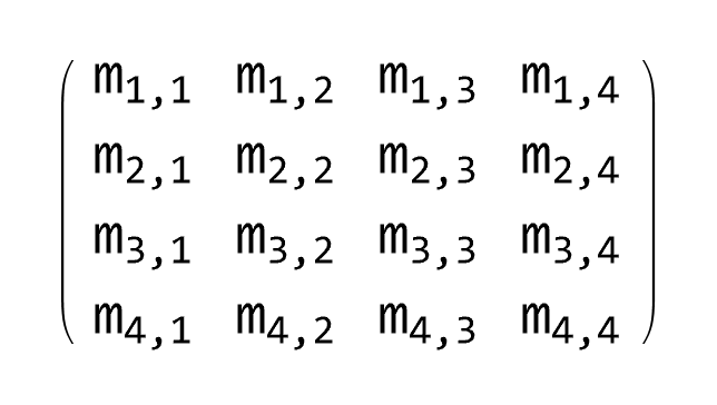
For this exercise to be consistent we need to establish a notation convention. Let's define a symbolic 4 x 4 matrix, M:

M = {{a, b, c, d}, {e, f, g, h}, {i, j, k, l}, {m, n, o, p}}
\( \displaystyle \begin{pmatrix} a& b& c& d \\ e& f& g& h \\ i& j& k& l \\ m& n& o& p \end{pmatrix} \)
Using the convention that the first character is the row number and the second character is the column number, we can double subscript the [lower case] elements of M. Mathematica needs to make these subscripted characters into an object. It does this with the "Symbolize" function in the Notation package.
<< Notation`;
Symbolize[ParsedBoxWrapper[SubscriptBox["_", "_"]]]; mSub = Table[Subscript[Symbol["m"], i, j], {i, 4}, {j, 4}]
\( \displaystyle \begin{pmatrix} m_{1,1}& m_{1,2}& m_{1,3}& m_{1,4} \\ m_{2,1}& m_{2,2}& m_{2,3}& m_{2,4} \\ m_{3,1}& m_{3,2}& m_{3,3}& m_{3,4} \\ m_{4,1}& m_{4,2}& m_{4,3}& m_{4,4} \end{pmatrix} \)
Here is a two-frame animation that cycles the symbolic and numeric repeatedly. Remember the numbers are from our original matrix, A. Notice the pattern of the subscripts as you read left-to-right in a single row; then notice the pattern as you read top-to-bottom in a single column; finally, notice the pattern along the main diagonal from upper left corner to lower right corner.
anim1 = Animate[ MatrixForm[ MapIndexed[ Function[{value, index}, Subscript[a, Sequence @@ index] = value; Subscript[element, Sequence @@ index]], {{-2, 1, -1, 2}, {-1, 2, -1, 1}, {2, -4, 1, -1}, {3, 2, 1, -2}}, {2}]], {element, {m, a}, AppearanceElements -> "PlayButton"} ]

Having already checked the Determinant, we move to step 2: Calculate the matrix of minors. Each of the 16 cells in the original matrix, A, will have its element replaced by a particular Minor. To find that number, for each element in the matrix, remove the row and column it's in. The determinant of the resulting, smaller, matrix is the minor for that element.

Although Mathematica automatically computes the determinants of each element's minor and places those determinants in a matrix, we perform these operations manually. Once done, you will never want to do it again and you will appreciate use of a computer algebra system.

We need to create a 3x3 "matrix of minors". Imagine if, for each cell, you ignore the other values in the column and row for that cell you would have then remaining a smaller 3x3 matrix:
A1 = {A[[2]], A[[3]], A[[4]]};
A11 = A1[[All, 2 ;; 4]]
\( \displaystyle \begin{pmatrix} 2& -1& 1 \\ -4& 1& -1 \\ 2& 1& -2 \end{pmatrix} \)
Its determinant is
Det[A11]
2
Here is a visual of the minor for the upper left cell in the original matrix. That red square is to be replaced by the Determinant of the minor in the lower right corner. We start with the top left corner and delete first row and first column to generate 3 × 3 matrix
Grid[{{Red, " ", " ", " "}, {" ", " 2", " -1", " 1"}, {" ", " -4", " 1", " -1"}, {" ", " 2", " 1", " -2"}}, Frame -> All]
🟥
2 -1 1
-4 1 -1
2 1 -2

The second Minor (Subscript[A, 1,2]) is evaluated as folows. Next, we eliminate the first row and second column from matrix A.

Grid[{{" ", Red, " ", " "}, {" -1 ", " ", " -1", " 1"}, {" 2 ", " ", " 1", " -1"}, {" 3 ", " ", " 1", " -2"}}, Frame -> All]
🟥
-1 -1 1
2 1 -1
3 1 -2

The corresponding matrix \[ {\bf A}_{12} = \begin{bmatrix} -1&-1&\phantom{-}1 \\ \phantom{-}2&\phantom{-}1&-1 \\ \phantom{-}3&\phantom{-}1&-2 \end{bmatrix} , \qquad \det {\bf A}_{12} = -1 , \] has determinant

Clear[Subscript[A, 1, 2]];
A1t = Transpose[A1];
A12 = Transpose[{A1t[[1]], A1t[[3]], A1t[[4]]}];
Det[A12]
-1
The next two minors corresponding the first row are \[ {\bf A}_{13} = \begin{bmatrix} -1&\phantom{-}2&-1 \\ \phantom{-}2&-4&-1 \\ \phantom{-}3&\phantom{-}2&-2 \end{bmatrix} , \qquad \det {\bf A}_{13} = 8, \]
🟥
-1 2 1
2 -4 -1
3 2 -2
A13 = Transpose[{A1t[[1]], A1t[[2]], A1t[[4]]}];
Det[A13]
8
and \[ {\bf A}_{14} = \begin{bmatrix} -1&\phantom{-}2&-1 \\ \phantom{-}2&-4&\phantom{-}1 \\ \phantom{-}3&\phantom{-}2&\phantom{-}1 \end{bmatrix} , \qquad \det {\bf A}_{14} = -8 . \]
🟥
-1 2 -1
2 -4 1
3 2 1
A14 = Transpose[{A1t[[1]], A1t[[2]], A1t[[3]]}];
Det[A14]
-8

Now we work out the second row.

Grid[{{" ", " 1", " -1", " 2"}, {Red, " ", " ", " "}, {" ", " -4", " 1", " -1"}, {" ", " 2", " 1", " -2"}}, Frame -> All]
1 -1 2
🟥
-4 1 -1
2 1 -2
A2 = {A[[1]], A[[3]], A[[4]]};
A21 = A2[[All, 2 ;; 4]]
\( \displaystyle \begin{pmatrix} 1& -1& 2 \\ -4& 1& -1 \\ 2& 1& -2 \end{pmatrix} , \qquad \det {\bf A}_{2,1} = -3 \)
Its determinant is
Det[A21]
-3

Minor for (2, 2)-cell is

Grid[{{" -2 ", " ", " -1", " 2"}, {" ", Red, " ", " "}, {" 2 ", " ", " 1", " -1"}, {" 3 ", " ", " 1", " -2"}}, Frame -> All]
-2 -1 2
🟥
2 1 -1
3 1 -2
A2 = {A[[1]], A[[3]], A[[4]]};
A2t = Transpose[A2];
A22 = Transpose[{A2t[[1]], A2t[[3]], A2t[[4]]}];
Det[A22]
-1
\[ {\bf A}_{22} = \begin{bmatrix} -2&-1&2 \\ 2&1&-1 \\ 3&1&-2 \end{bmatrix} , \qquad \det {\bf A}_{22} = -1 . \]

Similarly, we have

Grid[{{" -2 ", " 1", " ", " 2"}, {" ", " ", Red, " "}, {" 2 ", " -4", " ", " -1"}, {" 3 ", " 2", " ", " -2"}}, Frame -> All]
-2 1 2
🟥
2 -4 -1
3 2 -2
A2 = {A[[1]], A[[3]], A[[4]]};
A2t = Transpose[A2];
A23 = Transpose[{A2t[[1]], A2t[[2]], A2t[[4]]}];
Det[A23]
13
\[ {\bf A}_{2,3} = \begin{bmatrix} -2 & 1 & 2 \\ 2&-4& -1 \\ 3&2&-2 \end{bmatrix} , \qquad \det {\bf A}_{2,3} = 13 , \]
Grid[{{" -2 ", " 1", " -1", " "}, {" ", " ", " ", Red}, {" 2 ", " -4", " 1 ", " "}, {" 3 ", " 2", " 1", " "} }, Frame -> All]
-2 1 -1
🟥
2 -4 1
3 2 1
A2 = {A[[1]], A[[2]], A[[3]]};
A2t = Transpose[A2];
A24 = Transpose[{A2t[[1]], A2t[[2]], A2t[[3]]}];
Det[A24]
-3
\[ {\bf A}_{2,4} = \begin{bmatrix} -2 & 1 & -1 \\ 2&-4& 1 \\ 3&2&1 \end{bmatrix} , \qquad \det {\bf A}_{2,4} = -3 , \]

Reaching the halfway point, we can again check against Mathematica's built in function at this stage. First, let's assemble our individual minors.

{{Subscript[A, 1, 1], Subscript[A, 1, 2], Subscript[A, 1, 3], Subscript[A, 1, 4]}, {Subscript[A, 2, 1], Subscript[A, 2, 2], Subscript[A, 2, 3], Subscript[A, 2, 4]}}
\( \displaystyle \begin{pmatrix} 2& -1& 8& -8 \\ -3& -1& 13& -3 \end{pmatrix} \)
There is some consistency, albeit little. Notice the 2 x 4 matrix above is the reverse and reordered of the last two lines in the 4 x 4 matrix below
Minors[A]
\( \displaystyle \begin{pmatrix} 3& -3& 1& -2 \\ -2& -3& 1& 3 \\ -3& 13& -1& -3 \\ -8& 8& -1& 2 \end{pmatrix} \)
We can force them to match
{Reverse[Minors[A][[4]]], Reverse[Minors[A][[3]]]}
\( \displaystyle \begin{pmatrix} 2& -1& 8& -8 \\ -3& -1& 13& -3 \end{pmatrix} \)

The ninth Minor - third row, first column is

Grid[{{" ", " 1", " -1", " 2"}, {" ", " 2", " -1", " 1"}, {Red, " ", " ", " "}, {" ", " 2", " 1", " -2"}}, Frame -> All]
1 -1 2
2 -1 1
🟥
2 1 -2
\[ {\bf A}_{31} = \begin{bmatrix} 1&-1&\phantom{-}2 \\ 2&-1&\phantom{-}1 \\ 2& \phantom{-}1&-2 \end{bmatrix} , \qquad \det {\bf A}_{31} = 3, \]
Det[{{1, -1, 2},{2, -1, 1},{2, 1, -2}}]
3
Grid[{{" -2 ", " ", " -1", " 2"}, {" -1 ", " ", " -1", " 1"}, {" ", Red, " ", " "}, {" 3 ", " ", " 1", " -2"}}, Frame -> All]
-2 -1 2
-1 -1 1
🟥
3 1 -2
\[ {\bf A}_{32} = \begin{bmatrix} -2& -1& \phantom{-}2 \\ -1& -1& \phantom{-}1 \\ \phantom{-}3& \phantom{-}1& -2 \end{bmatrix} , \qquad \det {\bf A}_{32} = 1, \]
Det[{{-2, -1, 2}, {-1, -1, 1}, {3, 1, -2}}]
1
Grid[{{" -2 ", " 1", " ", " 2"}, {" -1 ", " 2", " ", " 1"}, {" ", " ", Red, " "}, {" 3 ", " 2", " ", " -2"}}, Frame -> All]
-2 1 2
-1 2 1
🟥
3 2 -2
\[ {\bf A}_{33} = \begin{bmatrix} -2&1&\phantom{-}2 \\ -1&2&\phantom{-}1 \\ \phantom{-}3&2&-2 \end{bmatrix} , \qquad \det {\bf A}_{33} = -3 , \]
Det[{{-2, 1, 2}, {-1, 2, 1}, {3, 2, -2}}]
-3
Grid[{{" -2 ", " 1", " -1", " "}, {" -1", " 2", " -1 ", " "}, {" ", " ", " ", Red}, {" 3 ", " 2", " 1", " "} }, Frame -> All]
-2 1 -1
-1 2 -1
🟥
3 2 1
The twelfth Minor - third row, fourth column is \[ {\bf A}_{34} = \begin{bmatrix} -2&1&-1 \\ -1&2&\phantom{-}1 \\ \phantom{-}3&2&\phantom{-}1 \end{bmatrix} , \qquad \det {\bf A}_{34} = -2 , \]
Det[{{-2, 1, -1}, {-1, 2, -1}, {3, 2, 1}}]
-2
The thirteenth Minor - fourth row, first column (Subscript[A, 4,1]) is
Grid[{{" ", " 1", " -1", " 2"}, {" ", " 2", " -1", " 1"}, {" ", " -4", " 1", " -1"}, {Red, " ", " ", " "}}, Frame -> All]
1 -1 2
-4 1 -1
2 1 -2
🟥
\[ {\bf A}_{41} = \begin{bmatrix} \phantom{-}1&-1&\phantom{-}2 \\ \phantom{-}2&-1&\phantom{-}1 \\ -4&\phantom{-}1&-1 \end{bmatrix} , \qquad \det {\bf A}_{41} = -2 , \]
Det[{{1, -1, 2}, {2, -1, 1}, {-4, 1, -1}}
-2
Grid[{{" -2 ", " ", " -1", " 2"}, {" -1 ", " ", " -1", " 1"}, {" 2 ", " ", " 1", " -1"}, {" ", Red, " ", " "}}, Frame -> All]
-2 -1 2
-1 -1 1
2 1 -1
🟥
\[ {\bf A}_{42} = \begin{bmatrix} -2&-1&\phantom{-}2 \\ -1&-1&\phantom{-}1 \\ \phantom{-}2&\phantom{-}1&-1 \end{bmatrix} , \qquad \det {\bf A}_{42} = 1 , \]
Det[{{-2, -1, 2}, {-1, -1, 1}, {2, 1, -1}}]
1
The fifteenth Minor - fourth row, third column (Subscript[A, 4,3]) is
Grid[{{" -2 ", " 1", " ", " 2"}, {" -1 ", " 2", " ", " 1"}, {" 2 ", " -4", " ", " -1"}, {" ", " ", Red, " "}}, Frame -> All]
-2 1 2
-1 2 1
2 -4 -1
🟥
\[ {\bf A}_{43} = \begin{bmatrix} -2&\phantom{-}1&\phantom{-}2 \\ -1&\phantom{-}2&\phantom{-}1 \\ \phantom{-}2&-4&-1 \end{bmatrix} , \qquad \det {\bf A}_{43} = -3 , \]
Det[{{-2, 1, 2}, {-1, 2, 1}, {2, -4, -1}}]
-3
The sixteenth Minor - fourth row, fourth column (Subscript[A, 4,4]) is
Grid[{{" -2 ", " 1", " -1", " "}, {" -1", " 2", " -1 ", " "}, {" 2 ", " -4", " 1", " "}, {" ", " ", " ", Red} }, Frame -> All]
-2 1 -1
-1 2 -1
2 -4 1
🟥
\[ {\bf A}_{44} = \begin{bmatrix} -2&\phantom{-}1&-1 \\ -1&\phantom{-}2&-1 \\ \phantom{-}2&-4&\phantom{-}1 \end{bmatrix} , \qquad \det {\bf A}_{44} = 3 . \]
Det[{{-2, 1, -1}, {-1, 2, -1}, {2, -4, 1}}]
3

Finally, we are now in a position to make the matrix of minors for our original matrix A based on the names we have given each one. We than can compare it with the built-in Mathematica code for Minors[ ]:

minMat = {{Subscript[A, 1, 1], Subscript[A, 1, 2], Subscript[A, 1, 3], Subscript[A, 1, 4]}, {Subscript[A, 2, 1], Subscript[A, 2, 2], Subscript[A, 2, 3], Subscript[A, 2, 4]}, {Subscript[A, 3, 1], Subscript[A, 3, 2], Subscript[A, 3, 3], Subscript[A, 3, 4]}, {Subscript[A, 4, 1], Subscript[A, 4, 2], Subscript[A, 4, 3], Subscript[A, 4, 4]}}
\( \displaystyle \begin{pmatrix} 2& -1& 8& -8 \\ -3& -1& 13& -3 \\ 3& 1& -3& -2 \\ -2& 1& -3& 3 \end{pmatrix} \)
\[ {\bf M} = \begin{bmatrix} \phantom{-}2&-1& \phantom{-}8&-8 \\ -3&-1&13 &-3 \\ \phantom{-}3&\phantom{-}1&-3&-2 \\ -2&\phantom{-}1&-3&\phantom{-}3 \end{bmatrix} . \]

With some machinations we can force Mathematica to agree with us!

Minors[A]
\( \displaystyle \begin{pmatrix} 3& -3& 1& -2 \\ -2& -3& 1& 3 \\ -3& 13& -1& -3 \\ -8& 8& -1& 2 \end{pmatrix} \)
Or, we can achieve the same answer by contorting our matrix of minors (minMat) equivalently.
Reverse[Reverse[#] & /@ minMat]
\( \displaystyle \begin{pmatrix} 3& -3& 1& -2 \\ -2& -3& 1& 3 \\ -3& 13& -1& -3 \\ -8& 8& -1& 2 \end{pmatrix} \)

3. Co-factor the matrix of minors. Apply a checkerboard of minuses to the "Matrix of Minors". Starting with a plus for the top left, alternate plus and minus through the matrix.

coFac = minMat*{{1, -1, 1, -1}, {-1, 1, -1, 1}, {1, -1, 1, -1}, {-1, 1, -1, 1}}
\( \displaystyle \begin{pmatrix} 2& 1& 8& 8 \\ 3& -1& -13& -3 \\ 3& -1& -3& 2 \\ 2& 1& 3& 3 \end{pmatrix} \)
\[ \mbox{Co-factors} = \begin{bmatrix} \phantom{-}2&1& \phantom{-}8&8 \\ 3&-1&-13 &-3 \\ \phantom{-}3&-1&-3&2 \\ 2&\phantom{-}1&3&\phantom{-}3 \end{bmatrix} . \]

4. Transpose the co-factor matrix. Swap the elements of the rows and columns.

\[ \mbox{Co-factors}^{\mathrm T} = \begin{bmatrix} 2&\phantom{-}3& \phantom{-}3&2 \\ 1&-1&-1 &1 \\ 8&-13&-3&3 \\ 8& -3&\phantom{-}2&3 \end{bmatrix} . \]
adjA = coFac\[Transpose]
\( \displaystyle \begin{pmatrix} 2& 3& 3& 2 \\ 1& -1& -1& 1 \\ 8& -13& -3& 3 \\ 8& -3& 2& 3 \end{pmatrix} \)

5. Divide each element of the transposed matrix by the determinant. This will result in the inverse of the original matrix.

invA = adjA/Det[A] // N
\( \displaystyle \begin{pmatrix} 0.4& 0.6& 0.6& 0.4 \\ 0.2& -0.2& -0.2& 0.2 \\ 1.6& -2.6& -0.6& 0.6 \\ 1.6& -0.6& 0.4& 0.6 \end{pmatrix} \)
We compare our answer with the answer provided by Mathematica:
invA == Inverse[A] // N
True
\[ \mbox{Adjugate} = \left( \det {\bf A} \right) {\bf A}^{-1} = \begin{bmatrix} 2& \phantom{-}3& \phantom{-}3& 2 \\ 1& -1& -1& 1 \\ 8& -13& -3& 3 \\ 8& -3& \phantom{-}2& 3\end{bmatrix} . \]
End of Example 10

The formula for A−1 in the following theorem first appeared in a more general form in Arthur Cayley's Memoir on the Theory of Matrices.

Theorem 10: (A. Cayley, 1858) The inverse of a 2-by-2 matrix is given by the formula: \[ \begin{bmatrix} a&b \\ c&d \end{bmatrix}^{-1} = \frac{1}{ad-bc} \begin{bmatrix} \phantom{-}d&-b \\ -c&\phantom{-}a \end{bmatrix} , \qquad ad \be bc . \]

Theorem 11: The inverse of a square matrix A is the transpose of the cofactor matrix times the reciprocal of the determinant of A:

\[ {\bf A}^{-1} = \frac{1}{\det\,{\bf A}} \,\mbox{adj}\,{\bf A} = \frac{1}{\det\,{\bf A}} \,{\bf C}^{\mathrm T} , \qquad\mbox{where} \quad {\bf C} = \begin{bmatrix} C_{1,1} & C_{1,2} & \cdots & C_{1,n} \\ C_{2,1} & C_{2,2} & \cdots & C_{2,n} \\ \vdots&\vdots& \ddots & \vdots \\ C_{n,1} & C_{n,2} & \cdots & C_{n,n} \end{bmatrix} \]
is the cofactor matrix (also called the matrix of cofactors).

Algorithm for calculating inverse matrix using Theorem 11: The inverse of a square matrix A is obtained by performimh four steps:

  1. Calculating the matrix of Minors; namely, for each entry of the matrix A:
    • ignore the values on the current row and column,
    • calculate the determinant of the matrix built from the remaining values.
    Put those determinants into a matrix (the "matrix of Minors").
  2. Then turn matrix of Minors into the matrix of Cofactors. This means that you need to multiply every (i, j)-entry of the matrix of Minors by (−1)i + j.
  3. Calculate the Adjugate to A, denoted as Adj(A). This requires to apply transposition to the matrix of Cofactors.
  4. Multiply the Adjugate matrix by the reciprocal of the determinant of A.
Our starting point is the cofactor expansion:
\[ \det {\bf A} = \sum a_{i,k}\,A_{j,k} , \]
where Aj,k is the cofactor of the element aj,k, and the sum is either on j (for any fixed value of k) or on k (for any fixed value of j). If we have the sum over j, then
\[ \sum_j a_{j,k} A_{j,i} = \begin{cases} \det {\bf A} , & \ \mbox{ if } \ i=k , \\ 0, & \ \mbox{ if } \ i \ne k \end{cases} \]
since we get two identical columns when ik. Upon division by det A, we have
\[ \sum_j \left( \frac{A_{j,i}}{\det {\bf A}} \right) a_{j,k} = \delta_{i,k} = \begin{cases} 1 , & \ \mbox{ if } \ i=k , \\ 0, & \ \mbox{ if } \ i \ne k . \end{cases} \]
This scalar statement (which holds for \( 1 \le i \le n, \ 1 \le j \le n \) ) is equivalent, according to the definition of matrix multiplication to the matrix equation
\[ {\bf A}^{-1} {\bf A} = {\bf I}_n , \]
where the desired inverse matrix is
\[ {\bf A}^{-1} = \left[ \frac{A_{j,i}}{\det {\bf A}} \right] . \]
Example 11: We start with a general 2 × 2 matrix:
\[ \begin{bmatrix} a&b \\ c&d \end{bmatrix}^{-1} = \frac{1}{ad-bc} \,\begin{bmatrix} d&-b \\ -c&a \end{bmatrix} , \]
eq1 = a*alpha + b*gamma == 1
eq2 = a*beta + b*delta == 0
eq3 = c*alpha + d*gamma == 0
eq4 = c*beta + d*delta == 1
Solve[{eq1, eq2, eq3, eq4}, {alpha, beta, gamma, delta}]
{{alpha -> d/(-b c + a d), beta -> b/(b c - a d), gamma -> c/(b c - a d), delta -> a/(-b c + a d)}}
and
\[ \begin{bmatrix} a_{11}&a_{12}&a_{13} \\ a_{21}&a_{22}&a_{23} \\ a_{31}&a_{32} &a_{33} \end{bmatrix}^{-1} = \frac{1}{\det\,{\bf A}} \,\begin{bmatrix} \begin{vmatrix} a_{22}&a_{23} \\ a_{32}&a_{33} \end{vmatrix}& \begin{vmatrix} a_{13}&a_{12} \\ a_{33}&a_{32} \end{vmatrix} & \begin{vmatrix} a_{12}&a_{13} \\ a_{22}&a_{23} \end{vmatrix} \\ \begin{vmatrix} a_{23}&a_{21} \\ a_{33}&a_{31} \end{vmatrix}&\begin{vmatrix} a_{11}&a_{13} \\ a_{31}&a_{33} \end{vmatrix} &\begin{vmatrix} a_{13}&a_{11} \\ a_{23}&a_{21} \end{vmatrix} \\ \begin{vmatrix} a_{21}&a_{22} \\ a_{31}&a_{32} \end{vmatrix} & \begin{vmatrix} a_{12}&a_{11} \\ a_{32}&a_{31} \end{vmatrix} & \begin{vmatrix} a_{11}&a_{12} \\ a_{21}&a_{22} \end{vmatrix} \end{bmatrix} , \]
where we use the vertical lines to define determinants of corresponding matrices.
A = {{a,b,c}, {d,e,f}, {g,h,i}};
K = {{p,q,r}, {u,v,w}, {x,y,z}};
P = A.K;
Solns = Simplify[Solve[{P == IdentityMatrix[3]}, {p,q,r,u,v,w,x,y,z}]]

The cofactor matrix can be computed in the Wolfram language using

Cofactor[m_List?MatrixQ, {i_Integer, j_Integer}] :=
(-1)^(i+j) Det[Drop[Transpose[
Drop[Transpose[m], {j}]], {i} ]]
which is the equivalent of the (i,j)-th components of the CofactorMatrix defined below:
MinorMatrix[m_List?MatrixQ] :=
Map[Reverse, Minors[m], {0, 1}]
CofactorMatrix[m_List?MatrixQ] :=
MapIndexed[#1 (-1)^(Plus @@ #2)&, MinorMatrix[m],{2}]
End of Example 11

Corollary 2: A square matrix A is invertible (nonsingular) if and only if its determinant det(A) ≠ 0.

Example 12: Consider the matrix
\[ {\bf A} = \begin{bmatrix} 48&-30&-14&1 \\ 65&-41&-19&0 \\ 17&-10&-5&3 \\ -35&22&10&0 \end{bmatrix} . \]
To find its inverse, we need to check whether the given matrix is singular or not:
A = {{48, -30, -14, 1}, {65, -41, -19, 0}, {17,-10,-5,3}, {-35, 22, 10, 0}}
Det[A]
Out[2]= -1
Now we calculate the cofactor matrix:
\begin{align*} C_{1,1} &= \det \begin{bmatrix} -41&-19&0 \\ -10&-5&3 \\ 22&10&0 \end{bmatrix} = -24 , \\ C_{1,2} &= - \det \begin{bmatrix} 65&-19&0 \\ 17&-5&3 \\ -35&10&0 \end{bmatrix} = -45, \\ C_{1,3} &= \det \begin{bmatrix} 65&-41&0 \\ 17&-10&3 \\ -35&22&0 \end{bmatrix} = 15, \\ C_{1,4} &= - \det \begin{bmatrix} 65&-41&-19 \\ 17&-10&-5 \\ -35&22&10 \end{bmatrix} = -11. \end{align*}
Similarly, we can calculate all other cofactors, which yields, together with \( \det{\bf A} = -1 , \) the inverse matrix:
\[ {\bf A}^{-1} = \begin{bmatrix} 24&-14&-8&3 \\ 45&-25&-15&8 \\ -15&6&5&-7 \\ -11&6&4&-2 \end{bmatrix} . \]
End of Example 12

 Now we compute the inverse matrix based on our knowledge how to solve systems of linear equations! If A is an n × n nonsingular matrix, then for any column vector b, which is n × 1 matrix, the linear system A x = b has a unique solution. Partition the identity matrix In into its columns that we denote as \( {\bf e}_i , \ i=1,2,\ldots , n . \) Since the identity matrix can be represented as an array of column-vectors \( {\bf I}_n = \left[ {\bf e}_1 \ {\bf e}_2 \ \cdots \ {\bf e}_n \right] , \) every linear equation \( {\bf A}\,{\bf x} = {\bf e}_i \) has a unique solution for each i. Hence, we have

\[ {\bf A}\,{\bf c}_1 = {\bf e}_1 , \quad {\bf A}\,{\bf c}_2 = {\bf e}_2 , \quad \cdots \quad {\bf A}\,{\bf c}_n = {\bf e}_n , \]
Writing the above system of equations in matrix form, we get
\[ \left[ {\bf A}\,{\bf c}_1 , \ {\bf A}\,{\bf c}_2 , \ \cdots \ {\bf A}\,{\bf c}_n \right] = \left[ {\bf e}_1 \ {\bf e}_2 \ \cdots \ {\bf e}_n \right] = {\bf I}_n . \]
From our observation on partitioned matrices, the above matrix equation can be written in the form
\[ {\bf A} \left[ {\bf c}_1 , \ {\bf c}_2 , \ \cdots \ {\bf c}_n \right] = {\bf I}_n . \]
Letting \( {\bf C} = \left[ {\bf c}_1 , \ {\bf c}_2 , \ \cdots \ {\bf c}_n \right] , \) we have just shown that C is the inverse of A.
Example 13: Suppose we need to find the inverse of the matrix
\[ {\bf A} = \begin{bmatrix} \phantom{-}2 & 1 & 1 \\ -2& 3 &9 \\ -1&0& 1 \end{bmatrix} . \]
A = {{2, 1, 1}, {-2, 3, 9}, {-1, 0, 1}}
Of course, Mathematica finds its inverse in a blank of eye:
Inverse[A]
{{3/2, -(1/2), 3}, {-(7/2), 3/2, -10}, {3/2, -(1/2), 4}}
\[ {\bf A}^{-1} = \frac{1}{2} \begin{bmatrix} \phantom{-}3&-1&6 \\ -7&\phantom{-}3&-20 \\ \phantom{-}3&-1&8 \end{bmatrix} . \tag{13.1} \] We determine every column in the latter by solving three systems of equations: \[ \begin{split} 2\, x_1 + x_2 + x_3 &= 1, \\ -2\, x_1 + 3\, x_2 + 9\, x_3 &= 0 , \\ -x_1 + x_3 &= 0 ; \end{split} \tag{13.2} \] According to the theory, to solve system of equations (13.2), we build the augmented matrix \[ \left[ {\bf A} \mid {\bf b} \right] = \begin{bmatrix} \phantom{-}2 & 1 & 1&1 \\ -2& 3 &9&0 \\ -1&0& 1&0 \end{bmatrix} . \] Then we use elementary row operations to reduce the augmented matrix to upper traingular form. \[ \left[ {\bf A} \mid {\bf b} \right] \,\underset{R}{\sim}\,\begin{bmatrix} 2 & 1 & 1&1 \\ 0& 4 &10&1 \\ 0&\frac{1}{2}& \frac{3}{2}&\frac{1}{2} \end{bmatrix} \,\underset{R}{\sim}\,\begin{bmatrix} 2 & 1 & 1&1 \\ 0& 4 &10&1 \\ 0&0& \frac{1}{4}&\frac{3}{8} \end{bmatrix} . \] Therefore, system of equations (13.2) is equivalent to \[ \begin{split} 2\, x_1 + x_2 + x_3 &= 1, \\ 4\, x_2 + 10\, x_3 &= 1 , \\ \frac{1}{4}\, x_3 &= \frac{3}{8} . \end{split} \] From the last equation, we immediately read off x₃ = 3/2. Substituting this value into the rest two equations, we get \[ \begin{split} 2\, x_1 + x_2 + \frac{3}{2} &= 1, \\ 4\, x_2 + 10\, \frac{3}{2} &= 1 , \end{split} \qquad \Longrightarrow \qquad \begin{split} 2\, x_1 + x_2 &= -\frac{1}{2}, \\ 4\, x_2 &= -14 . \end{split} \] Hence, the second unknown becomes x₂ = −7/2, which we use to determine the last one \[ 2\, x_1 - \frac{7}{2} = - \frac{1}{2} \qquad \Longrightarrow \qquad x_1 = \frac{3}{2} . \] Finally, we obtain the first column of the inverse matrix A−1 to be \[ {\bf c}_1 = \frac{1}{2}\,\begin{bmatrix} 3 \\ -7 \\ 3 \end{bmatrix} . \]
Subscript[c, 1] = Solve[{2*Subscript[x, 1] + Subscript[x, 2] + Subscript[x, 3] == 1, 4*Subscript[x, 2] + 10*Subscript[x, 3] == 1, Subscript[x, 3]/4 == 3/8}, {Subscript[x, 1], Subscript[x, 2], Subscript[x, 3]}]
{{x1 -> 3/2, x2 -> -(7/2), x3 -> 3/2}}
Then we come to the second system of equations: \[ \begin{split} 2\, x_1 + x_2 + x_3 &= 0, \\ -2\, x_1 + 3\, x_2 + 9\, x_3 &= 1 , \\ -x_1 + x_3 &= 0 ; \end{split} \tag{13.3} \] Determination of its solution we deligate to Mathematica:
Solve[{2*x1 + x2 + x3 == 0, -2*x1 + 3*x2 + 9*x3 == 1, -x1 + x3 == 0}, {x1, x2, x3}]
{{x1 -> -(1/2), x2 -> 3/2, x3 -> -(1/2)}}
So the second column of the inverse matrix becomes \[ {\bf c}_2 = \frac{1}{2}\,\begin{bmatrix} -1 \\ 3 \\ -1 \end{bmatrix} . \] We similarly solve the system \[ \begin{split} 2\, x_1 + x_2 + x_3 &= 0, \\ -2\, x_1 + 3\, x_2 + 9\, x_3 &= 0 , \\ -x_1 + x_3 &= 1 ; \end{split} \tag{13.4} \]
Solve[{2*x1 + x2 + x3 == 0, -2*x1 + 3*x2 + 9*x3 == 0, -x1 + x3 == 1}, {x1, x2, x3}]
{{x1 -> 3, x2 -> -10, x3 -> 4}}
Hence, the last column becomes \[ {\bf c}_3 =\begin{bmatrix} 3 \\ -10 \\ 4 \end{bmatrix} . \] Finally, we build the inverse matrix from these column vectors: \[ {\bf A}^{-1} = \left[ {\bf c}_1 \ {\bf c}_2 \ {\bf c}_3 \right] . \]
Transpose[{Subscript[c, 1][[1, All, 2]], Subscript[c, 2][[1, All, 2]], Subscript[c, 3][[1, All, 2]]}]
\( \displaystyle \begin{pmatrix} 3/2& -(1/2)& 3 \\ -(7/2)& 3/2& -10 \\ 3/2& -(1/2)& 4 \end{pmatrix} \)
% == Inverse[A]
True
End of Example 13

The inverse matrix can be determined using the resolvent method (see Chapter 8 in Dobrushkin's book for detail), which is based on the formula:

\begin{equation} \label{EqInverse.3} {\bf A}^{-1} = \sum_{\lambda_k \in \sigma (A)} \mbox{Res}_{\lambda_k} \lambda^{-1} {\bf R}_{\lambda} ({\bf A}) , \end{equation}
where summation is taken over all eigenvalues of matrix A, Resλ(f) is the residue of f at point λ, and Rλ = (λIA)−1 is the resolvent of matrix A.
Example 14: Let us consider the defective 4 × 4 matrix \[ {\bf B} = \begin{bmatrix} -115& 17& -85& -15 \\ -62& 11& -45& -8 \\ 124& -18& 92& 16 \\ 130& -19& 95& 18 \end{bmatrix} . \tag{14.1} \] First, we find its resolvent using Mathematica
R = Inverse[s*IdentityMatrix[4] - B]
{{(146 - 119 s + s^2)/(-2 + 5 s - 4 s^2 + s^3), (-21 + 17 s)/(-2 + 5 s - 4 s^2 + s^3), (105 - 85 s)/(-2 + 5 s - 4 s^2 + s^3), ( 19 - 15 s)/(-2 + 5 s - 4 s^2 + s^3)}, {( 76 - 62 s)/(-2 + 5 s - 4 s^2 + s^3), (-10 + 7 s + s^2)/(-2 + 5 s - 4 s^2 + s^3), (55 - 45 s)/(-2 + 5 s - 4 s^2 + s^3), ( 10 - 8 s)/(-2 + 5 s - 4 s^2 + s^3)}, {(-152 + 124 s)/(-2 + 5 s - 4 s^2 + s^3), ( 22 - 18 s)/(-2 + 5 s - 4 s^2 + s^3), (-109 + 88 s + s^2)/(-2 + 5 s - 4 s^2 + s^3), (-20 + 16 s)/(-2 + 5 s - 4 s^2 + s^3)}, {(-172 + 130 s)/(-2 + 5 s - 4 s^2 + s^3), ( 25 - 19 s)/(-2 + 5 s - 4 s^2 + s^3), (-125 + 95 s)/(-2 + 5 s - 4 s^2 + s^3), (-21 + 14 s + s^2)/(-2 + 5 s - 4 s^2 + s^3)}}
\[ {\bf R}_{\lambda}({\bf B}) = \left( \lambda {\bf I} - {\bf B} \right)^{-1} = \frac{m(\lambda )}{\left( \lambda -1 \right)^2 \left( \lambda -2 \right)} , \] where the numerator matrix in the resolvent formula is \[ m(\lambda ) = \begin{bmatrix} 146 - 119 \lambda + \lambda^2 & -21 + 17 \lambda & 105 - 85 \lambda & 19 - 15 \lambda \\ 76 - 62 \lambda & -10 + 7 \lambda + \lambda^2 & 55 - 45 \lambda & 10 - 8 \lambda \\ -152 + 124 \lambda & 22 - 18 \lambda &-109 + 88 \lambda + \lambda^2 & -20 + 16 \lambda \\ -172 + 130 \lambda & 25 - 19 \lambda & -125 + 95 \lambda & -21 + 14 \lambda + \lambda^2 \end{bmatrix} . \]
m[s_] = Simplify[Inverse[s*IdentityMatrix[4] - B]*(s-1)^2 *(s-2)]
Since the resolvent has two singular points λ = 1 and λ = 2, we need to find two residues at these points. We start with the first one. \[ \mbox{Res}_{\lambda =1} \frac{m(\lambda )}{\lambda \left( \lambda -1 \right)^2 \left( \lambda -2 \right)} = \lim_{\lambda \to 1} \frac{\text d}{{\text d}\lambda} \left( \frac{m(\lambda )}{\lambda \left( \lambda -2 \right)} \right) . \] This limit can be evaluated with the aid of Mathematica:
p=D[m[s]/s/(s-2),s] /.s->1
{{117, -17, 85, 15}, {62, -9, 45, 8}, {-124, 18, -90, -16}, {-130, 19, -95, -16}}
So the residue at λ = 1 becomes \[ {\bf P} = \begin{bmatrix} 117& -17& 85& 15 \\ 62& -9& 45& 8 \\ -124& 18& -90& -16 \\ -130& 19& -95& -16 \end{bmatrix} . \] The residue at another singular point is \[ \mbox{Res}_{\lambda =2} \frac{m(\lambda )}{\lambda \left( \lambda -1 \right)^2 \left( \lambda -2 \right)} = \lim_{\lambda \to 2} \frac{m(\lambda )}{\lambda \left( \lambda -1 \right)^2} = \frac{m(2)}{2} . \] Of course, this value is not hard to evaluate by hand, but lazy people like me deligate this job to software:
q=m[2]/2
{{-44, 13/2, -(65/2), -(11/2)}, {-24, 4, -(35/2), -3}, {48, -7, 71/2, 6}, {44, -(13/2), 65/2, 11/2}}
\[ \mbox{Res}_{\lambda =2} \frac{m(\lambda )}{\lambda \left( \lambda -1 \right)^2 \left( \lambda -2 \right)} = \begin{bmatrix} -44& 13/2& -(65/2)& -(11/2) \\ -24& 4& -(35/2)& -3 \\ 48& -7& 71/2& 6 \\ 44& -(13/2)& 65/2& 11/2 \end{bmatrix} . \] Adding these two expressions, we obtain the explicit expression for the inverse matrix:
q+p
{{73, -(21/2), 105/2, 19/2}, {38, -5, 55/2, 5}, {-76, 11, -(109/2), -10}, {-86, 25/2, -(125/2), -(21/2)}}
We compare this answer with the output provided by Mathematica when it was asked to find B−1:
Inverse[B]
{{73, -(21/2), 105/2, 19/2}, {38, -5, 55/2, 5}, {-76, 11, -(109/2), -10}, {-86, 25/2, -(125/2), -(21/2)}}
\[ {\bf B}^{-1} = \begin{bmatrix} 73 & - \frac{21}{2} & \frac{105}{2} & \frac{19}{2} \\ 38 & -5 & \frac{55}{2} & 5 \\ -76 & 11 & -\frac{109}{2} &-10 \\ -86 & \frac{25}{2} & - \frac{125}{2} &- \frac{21}{2} \end{bmatrix} . \]
End of Example 14
Example 15: Consider the spring-mass system that contains two masses m₁ and m₂ connecting with each other by a spring and also connected withe wall by two prings. This system is depicted below. Let x₁ and x₂ be displacements from the equilibrium positions of masses m₁ and m₂, respectively (with positive displacement being to the right). We assume that these masses are powered by forces f₁ and f₂, pointed positive when they act to the right.

coil1 = ParametricPlot[{t + 1.2*Sin[3*t], 1.2*Cos[3*t] - 1.2}, {t, -Pi/6, 5*Pi - Pi/6}, FrameTicks -> None, PlotStyle -> Black] ;
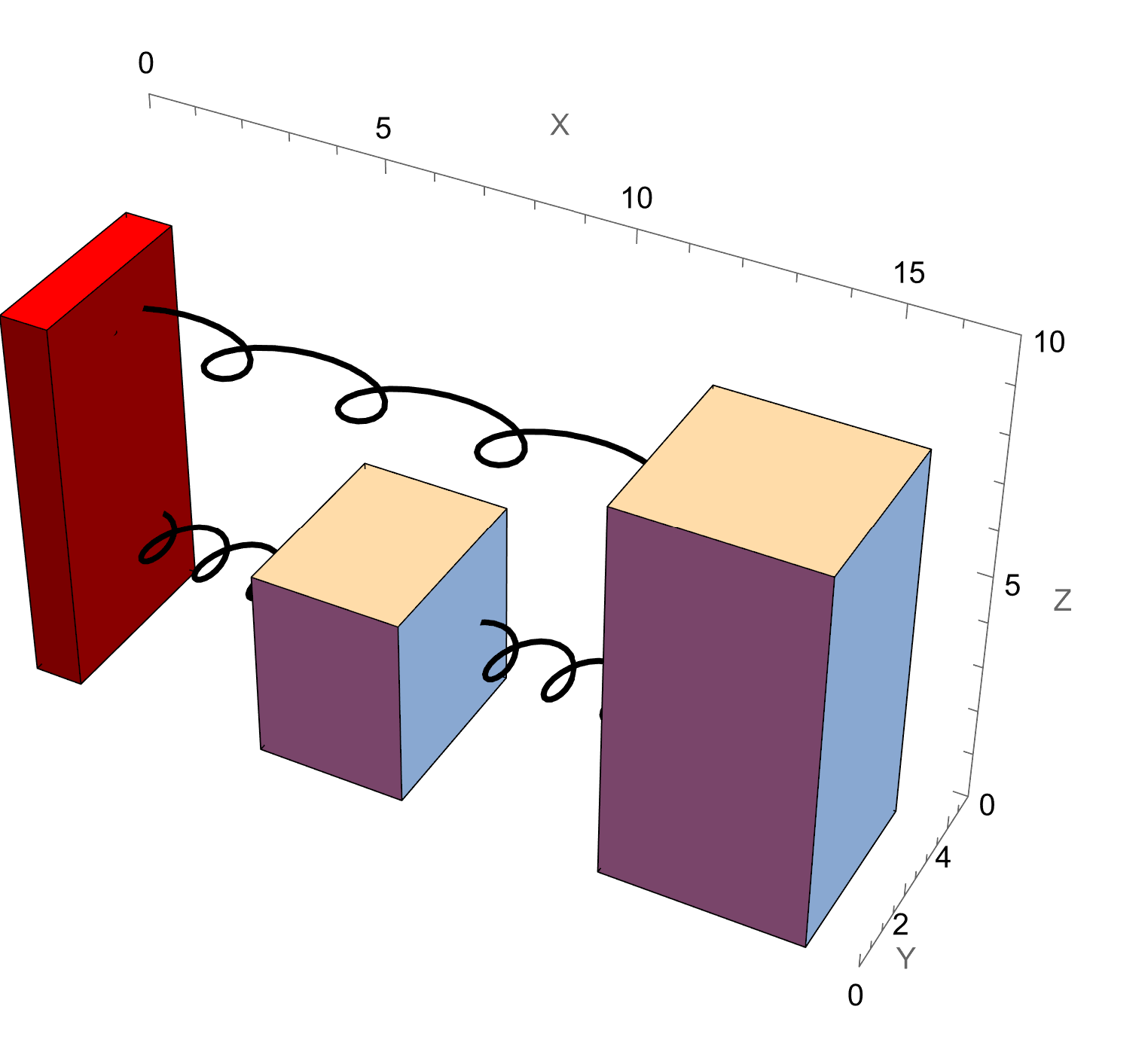
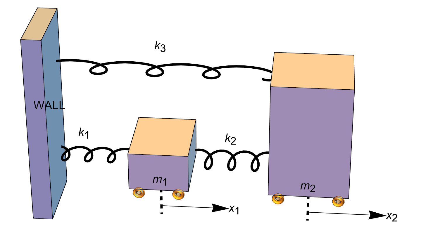
mass1 = Graphics[{Orange, Rectangle[{1, 0}, {1.5, 0.5}]}, AspectRatio -> 1] ;
mass2 = Graphics[{Pink, Rectangle[{3.0, 0}, {3.5, 2.0}]}, AspectRatio -> 1] ;

Two bodies inetraction
     
Two body system

According to Hooke’s Law, the force F required to stretch or compress a spring with spring constant k by a distance x is given by \[ F = k\,x . \] Taking into account the direction of force applied to each mass by the spring, we can write an equation for the force acting on each spring. The mass m₁ is being acted upon by two springs with spring constants k₁ and k₂. A displacement of x₁ by mass m₁ will cause the spring k₁ to stretch or compress depending on if x₁ is positive or negative. In either case, by Hooke’s Law, the force acting upon mass m₁ by spring k₁ is \[ - k_1 x_2 . \] We needed to include the negative sign as if x₁ were positive, then the force will need to be negative as the spring will be trying to pull the mass back.

How much spring k₂ will be stretched or compressed depends on displacements x₁ and x₂. In particular, it will be stretched by x₂ − x₂. Hence, the force acting on mass m₁ by spring k₂ is \[ k_2 \left( x_2 - x_1 \right) . \] For the system to be in equilibrium, the sum of the forces acting on mass m₁ must equal 0. Thus, we have \[ f_1 - k_1 x_1 + k_2 \left( x_2 - x_1 \right) = 0 . \]

Mass m₂ is being acted upon by springs k₂ and k₃. Using similar analysis, we find that \[ f_2 - k_3 x_2 -k_2 \left( x_2 - x_1 \right) = 0 . \] Rearranging this equations gives \[ \begin{split} k_1 x_1 + k_2 \left( x_1 - x_2 \right) &= f_1 , \\ k_2 \left( x_2 - x_1 \right) + k_3 x_2 &= f_1 . \end{split} \]

We want to find the forces f₁ and f₂ acting on the masses m₁ and m₂ given displacements x₁ and x₂. By Hooke’s Law, we find that the forces f₁ and f₂ satisfy Using matrix/vector multiplication, we can rewrite this system as \[ {\bf K}\,{\bf x} = {\bf f}, \qquad {\bf K} = \begin{bmatrix} k_1 + k_2 & - k_2 \\ -k_2 & k_2 + k_3 \end{bmatrix}, \quad {\bf x} = \begin{bmatrix} x_1 \\ x_2 \end{bmatrix}, \quad {\bf f} = \begin{bmatrix} f_1 \\ f_2 \end{bmatrix} . \] Matrix K is known as the stiffness matrix of the system. In order to find displacements, we multiply both sides of the latter equation by K−1 to obtain \[ {\bf K}^{-1} = \frac{1}{k_1 k_2 + k_1 k_3 + k_2 k_3} \begin{bmatrix} k_2 + k_3 & k_2 \\ k_2 & k_1 + k_2 \end{bmatrix} . \]

Inverse[{{k1 + k2, -k2}, {-k2, k2 + k3}}]
{{(k2 + k3)/(k1 k2 + k1 k3 + k2 k3), k2/( k1 k2 + k1 k3 + k2 k3)}, {k2/(k1 k2 + k1 k3 + k2 k3), (k1 + k2)/( k1 k2 + k1 k3 + k2 k3)}}
End of Example 15

  1. Anton, Howard (2005), Elementary Linear Algebra (Applications Version) (9th ed.), Wiley International
  2. Beezer, R.A., A First Course in Linear Algebra, 2017.
  3. Dobrushkin, V.A., Applied Differential Equations. The Primary Course, second edition, CRC Press2022.
  4. Fadeev--LeVerrier algorithm, Wikipedia.
  5. Frame, J.S., A simple recursion formula for inverting a matrix, Bulletin of the American Mathematical Society, 1949, Vol. 55, p. 1045. doi:10.1090/S0002-9904-1949-09310-2
  6. Greenspan, D., Methods of matrix inversion, The American mathematical Monthly, 1955, Vol. 62, No. pp. 303--318.
  7. Karlsson, L., Computing explicit matrix inverses by recursion, Master's Thesis in Computing Science, 2006.
  8. Lightstone, A.H., Two methods of inverting matrices, Mathematics Magazine, 1968, Vol. 41, No. 1, pp. 1--7.
Inverse Block Matrices