Elementary Reduction Operations

Example 1: We illustrate different approaches when solving the following underdetermined system of equations (when there are fewer equations than unknowns) \[ \begin{split} 2\,x_1 + 3\, x_2 + 5\, x_3 &= 3, \\ 3\,x_1 - 2\,x_2 - 2\, x_3 &= 1 . \end{split} \tag{1.1} \]

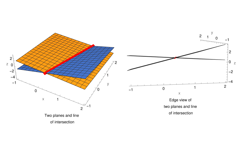
Each equation in (1.1) can be written as dot products a₁ • x = 3 and a₂ • x = 1, where \[ {\bf a}_1 = \left( 2, 3, 5 \right) , \quad {\bf a}_2 = \left( 3, -2, -2 \right) , \] and x = (x₁, x₂, x₃) ∈ ℝ³. The solution set of the equation a • x = b is also a plane in ℝ³.

Geometrically we expect that the intersection of two nonparallel planes in ℝ³ is a line. (If you hold out two sheets of paper and turn the sheets so that they are not parallel, their intersection is a line. Imagine that the sheets are extended forever and ever.) The equation of this line is \[ S = \left\{ \left[ \begin{array}{c} x_1 \\ x_2 \\ x_3 \end{array} \right] \in \mathbb{R}^{3\times 1} \ : \ 2\,x_1 + 3\, x_2 + 5\, x_3 = 3 \quad\mbox{and} \quad 3\,x_1 - 2\,x_2 - 2\, x_3 = 1 \right\} . \] In order to plot the intersection of these two planes, we use a trick by introducing new variables (x, y, and z) without indexing that are common in physics and engineering. Below on the left you see the two planes with their intersection line in red; on the right is the edge view of the same graphic where the line momentarily becomes a point.

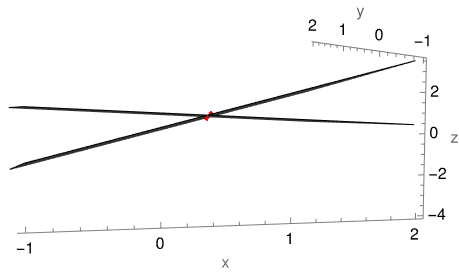
Intersection of two planes defines a line.		Edge view of two planes and line of intersection.

We know that a line is the set of points that can be written as the sum of a shift vector plus all scalar multiples of a nonzero vector (known as the generator). The set S does not look like a line. In fact, it is hard to look at S and tell if there are any points at all in S. To show that S is a line of points, we must resort to algebra and arithmetic, and solve the two defining equations simultaneously. In particular, to answer our question we must solve the system (1.1).

We convert the given row problem (1.1) into column problem. Let V ⊆ ℝ² be spanned on three vectors: \[ V = \mbox{span}\left\{ \begin{bmatrix} 2 \\ 3 \end{bmatrix} , \ \begin{bmatrix} \phantom{-}3 \\ -2 \end{bmatrix} , \ \begin{bmatrix} \phantom{-}5 \\ -2 \end{bmatrix} \right\} . \] V is a subspace of ℝ², and in fact, it is generated by linear combinations \[ V = \left\{ x_1 \begin{bmatrix} 2 \\ 3 \end{bmatrix} + x_2 \begin{bmatrix} \phantom{-}3 \\ -2 \end{bmatrix} + x_3 \begin{bmatrix} \phantom{-}5 \\ -2 \end{bmatrix} \ : \ x_1 , x_2 , x_3 \mbox{ are real numbers} \right\} . \] System of equations (1.1) has a solution iff the right-hand side vector \( \displaystyle {\bf b} = \begin{bmatrix} 3 \\ 1 \end{bmatrix} \) belongs to V: \[ \begin{bmatrix} 3 \\ 1 \end{bmatrix} = x_1 \begin{bmatrix} 2 \\ 3 \end{bmatrix} + x_2 \begin{bmatrix} \phantom{-}3 \\ -2 \end{bmatrix} + x_3 \begin{bmatrix} \phantom{-}5 \\ -2 \end{bmatrix} . \] Our immediate task is to solve the system of equations (1.1). So we ask Mathematica for help. First, we introduce new variables in order to distinguish our new approach with the previously one.

\[ x_1 = \frac{1}{13} \left( 9 - 4\, x_3 \right) , \quad x_2 = \frac{1}{13} \left( 7 - 19\, x_3 \right) \] How does Mathematica know the general solution ? To answer this question, we multiply the first equation by 2 and the second equation by 3; this leads to \[ \begin{split} 4\,x_1 + 6\, x_2 + 10\, x_3 &= 6, \\ 9\,x_1 - 6\,x_2 - 6\, x_3 &= 3 . \end{split} \] Upon adding these results, we eliminate variable x₂ because it is multiplied by zero: \[ \begin{split} 4\,x_1 + 6\, x_2 + 10\, x_3 &= 6, \\ 13\,x_1 + 0\,x_2 + 4\, x_3 &= 9 . \end{split} \tag{1.2} \] Solving the latter, we get \[ x_1 = \frac{1}{13} \left( 9 - 4\, x_3 \right) . \] Mathematica can accomplish that with one line of code. A detailed discussion of the line of code above is given below. However, at the risk of being pedantic, one can break up the code above into a number of steps, making it more readable and understandable. Back substitution x₁ into the first equation yields \[ \frac{2}{13} \left( 9 - 4\,x_3 \right) + 3\, x_2 + 5\, x_3 = 3 . \] This allows us to determine x₂ as a function of x₃. Since both unknowns x₁ and x₂ are expressed through x₃ can be considered x₃ as a free variable.

======================= Roger ==================

However, we can makes the system (1.2) looks nicer. In order to achive it, we use Chiò's method, invented by the Italian mathematician Felice Chiò (1813--1871) in 1853. At his time, computers wee not available and people did not (and still do not) feel comfortable working with fractions.

First, we observe that there is no need to continue writing the 'unknowns' x₁, x₂, x₃ because we work only with their coefficients. Therefore, we introduce vectors with corresponding coefficients that we abbreviate as \[ {\bf r}_1 = \begin{bmatrix} 2&3&5&3 \end{bmatrix} \qquad\mbox{and} \qquad {\bf r}_2 = \begin{bmatrix} 3&-2&-2&1 \end{bmatrix} . \] We multiply the first vector r₁ by 3 and subtract the second vectorr₂ multiplied by 2. This yields \[ 3\,{\bf r}_1 = \begin{bmatrix} 6&9&15&9 \end{bmatrix} \qquad\mbox{and} \qquad 2\,{\bf r}_2 = \begin{bmatrix} 6&-4&-4&2 \end{bmatrix} . \] So \[ {\bf w} = 3\,{\bf r}_1 - 2\,{\bf r}_2 = \begin{bmatrix} 0&13&19&7 \end{bmatrix} . \] Now we compare the second components of vectors w and r₂, we can make them equal upon multiplication w vt 2 and r₂, by 13: \[ 2\,{\bf w} = \begin{bmatrix} 0&26&38&14 \end{bmatrix} , \qquad 13\,{\bf r}_2 = \begin{bmatrix} 39&-26&-26&13 \end{bmatrix} . \] Adding these two vectors, we obtain \[ {\bf u} = 2\,{\bf w} + 13\,{\bf r}_2 = \begin{bmatrix} 39&0&12&27 \end{bmatrix} . \] Since system of equations corresponding vectors r₁ and r₂ is equivalent to the system of equations generated by vectors u and w, we claim that our system of equations is equivalent to the following system: \[ \begin{split} 0\,x_1 + 13\, x_2 + 19\, x_3 &= 7, \\ 39\,x_1 + 0\,x_2 + 12\, x_3 &= 27 . \end{split} \tag{1.4} \] Each of equations in (1.4) contains only two variables, so we can determine one of them: \[ 13\, x_2 = 7 - 19\, x_3 , \qquad 39\, x_1 = 27 - 12 \, x_3 \quad \iff \quad 13\, x_1 = 9 - 4\, x_ 3 . \] We can use the same approach eliminating variables in each equation of system (1.2). Again we start with vectors r₁ and r₂, but now eliminate variables x₁ and x₃. We can use vector w because its first component is zero. Comparing its third component (19) and the third component (−2) of r₂, we see that we need to build another vector \[ {\bf v} = 2\,{\bf w} + 19\,{\bf r}_2 = \begin{bmatrix} 39&12&0&33 \end{bmatrix} . \] Then the system of equations w, v contains only two unknown variables in equa equation \[ \begin{split} 0\,x_1 + 13\, x_2 + 19\, x_3 &= 7, \\ 39\,x_1 + 12\,x_2 + 0\, x_3 &= 33 . \end{split} \tag{1.5} \] Solving this system with respect to x₁ and x₃, we obtain \[ 13\, x_1 = 11 - 4\, x_2 , \qquad 19\, x_3 = 7 - 13\, x_ 2 , \] where x₂ is a free variable.

=================== to be checked ==============

\[ \begin{split} 0\,x_1 + 78\, x_2 + 114\, x_3 &= 42, \\ 13\,x_1 + 0\,x_2 + 4\, x_3 &= 9 . \end{split} \tag{1.3} \] We can simplify system (11.3) further by dividing each term in the first equation by 6. This gives us a nice system: \[ \begin{split} 0\,x_1 + 13\, x_2 + 19\, x_3 &= 7, \\ 13\,x_1 + 0\,x_2 + 4\, x_3 &= 9 . \end{split} \tag{1.4} \] The x₃ variable can simply be anything, so let x₃ = 13t. Then solution of Eq.(1.1) is expressed in the form of line in ℝ³: \[ \begin{bmatrix} x_1 \\ x_2 \\ x_3 \end{bmatrix} = \frac{1}{13} \begin{bmatrix} 9 \\ 7 \\ 0 \end{bmatrix} + t \begin{bmatrix} -4 \\ -19 \\ 13 \end{bmatrix} , \qquad t \in \mathbb{R} . \]

Now we multiply the first equation by 2 and the second one by 5. Upon adding the results, we obtain \[ \begin{split} 4\,x_1 + 6\, x_2 + 10\, x_3 &= 6, \\ 19\,x_1 - 4\,x_2 &= 11 . \end{split} \] Solving for x₁ and then substitute into the first equation, we get the general solution \[ x_1 = \frac{1}{19} \left( 11 + 4\, x_2 \right) , \quad x_3 = \frac{1}{19} \left( 7 - 13\, x_2 \right) \] We verify with Mathematica:

So now variable x₂ is free and two variables are expressed through it. Similarly, we can obtain the general solution that has x₁ as a free variable: \[ x_2 = \frac{1}{4} \left( -11 + 19\, x_1 \right) , \quad x_3 = \frac{1}{4} \left( 9 - 13\, x_1 \right) . \]

Example 2: Consider the simple 2 × 3 system \[ \begin{split} x - 2\,y + 3\,z &= -7, \\ 3\,x + 5\,y - 2\,z &= 23 . \end{split} \tag{4.1} \] The left-had side of the system defines a linear transformation T : 𝔽³ ⇾ 𝔽² via simple rule: \[ T(x, y, z) = \left( x - 2\,y + 3\,z , 3\,x + 5\,y - 2\,z \right) \in \mathbb{R}^2 . \] Therefore, solving this system means finding all inputs (x, y, z) from ℝ³ that are mapped by T into a "target" vector (−7, 23) ∈ ℝ². Any linear transformation can be rewritten in matrix/vector form A x = b, where \[ {\bf A} = \begin{bmatrix} 1 & -2 & \phantom{-}3 \\ 3 & \phantom{-}5 & -2 \end{bmatrix}, \qquad {\bf x} = \begin{pmatrix} x \\ y \\ z \end{pmatrix} , \quad {\bf b} = \begin{bmatrix} -7 \\ 23 \end{bmatrix} . \]

So we can also read the system as a problem about linear combinations of the columns of A. In this case, for instance, A x = b becomes a column problem \[ x \begin{pmatrix} 1 \\ 3 \end{pmatrix} + y \begin{pmatrix} -2 \\ 5 \end{pmatrix} + z \begin{pmatrix} 3 \\ -2 \end{pmatrix} = \begin{pmatrix} -7 \\ 23 \end{pmatrix} , \] or \[ x\,{\bf a}_1 + y\,{\bf a}_2 + z\,{\bf a}_2 = {\bf b} , \] where \[ {\bf a}_1 = \begin{pmatrix} 1 \\ 3 \end{pmatrix} , \quad {\bf a}_2 = \begin{pmatrix} -2 \\ 5 \end{pmatrix} , \quad {\bf a}_3 = \begin{pmatrix} 3 \\ -2 \end{pmatrix} \] denotes column j of matrix A. Seen in this light, solving the linear system means finding a linear combination of the vectors {a₁, a₂, a₃} that adds up to (−7, 23).

Each individual equation in the system (4.1) has the form r_i(A) • (x, y, z) = b_i, i = 1, 2, where r_i(A) denotes row i of A (and b_i is the ith entry in b ). In particular, \[ {\bf r}_1 ({\bf A}) = \left( 1, -2, 3 \right) , \quad {\bf r}_2 ({\bf A}) = \left( 3, 5, -2 \right) . \] We could write the 2-by-3 system (1.1) as \[ \begin{split} \left( 1, -2, 3 \right) \bullet (x, y, z) &= -7 , \\ \left( 3, 5, -2 \right) ) \bullet (x, y, z) &= 23 . \end{split} \] So from the row standpoint, the problem A x = b becomes: Find all vectors in ℝ³ (if any) that dot with each row of A to give the corresponding entry in b ∈ ℝ². This is the row problem. It is dual to the column problem.

Example 3: The system \[ \begin{split} x - 3\,y &= -1 , \\ 2\,x + y &= 12 , \end{split} \] has the solution (x, y) = (5, 2). Indeed, replacing 5 for x and 2 for y in each of the two equations, we have 5 − 3 × 2 = −1 and 2 × 5 + 2 = 12. Let us consider the generic linear combination of the equations of the system \[ c_1 \left( x - 3\,y \right) + c_2 \left( 2\,x + y \right) = -c_1 + 12\, c_2 \] and verify that this equation has the solution (5, 2); in fact, if (x, y) = (5, 2), we obtain \[ c_1 \left( 5 - 3 \cdot 2 \right) + c_2 \left( 2\cdot 5 + 2 \right) = -c_1 + 12\, c_2 . \]

Example 4: The system \[ \begin{split} E_1 \ : \quad 3\,x - y &= 0 , \\ E_2 \ : \, -x + 2\,y &= 5 , \\ E_3 \ : \ \ \phantom{-x +} 5\, y &= 15 , \end{split} \] is equivalent to the system of the last two equations because E₃ = E₁ + 3·E₂. Therefore, the system admits the unique solution (1, 3).

Example 5: We consider the following system of equations \[ \begin{array}{c} \mbox{E}_1 \ : \\ \mbox{E}_2 \ : \end{array} \qquad \begin{cases} \phantom{3\,}x_1 + 2\, x_2 + 3\, x_3 &= 2, \\ 3\,x_1 - 2\,x_2 - 2\, x_3 &= 1 . \end{cases} \tag{5.1} \] Let us add the first equation to the second one; this yields an equivalent system of equations \[ \begin{array}{c} \mbox{E}_1 \ : \\ \mbox{E}_1 + \mbox{E}_2 \ : \end{array} \qquad \begin{split} x_1 + 2\, x_2 + 3\, x_3 &= 2, \\ 4\,x_1 + 0\,x_2 + 1\, x_3 &= 3 . \end{split} \] However, the latter contains only two independent variables instead of initial three variables. This means that we eliminate one of the variables and reduce the dimension of the equation: equation 3·x₁ + x₃ = 3 is 1 × 2 equation.

For further simplification, we multiply the second equation by (−3) and add to the first one. As a result, we get \[ \begin{array}{c} \mbox{E}_1 - 3\left( \mbox{E}_1 + \mbox{E}_2 \right) \ : \\ \mbox{E}_1 + \mbox{E}_2 \ : \end{array} \qquad \begin{split} -11\,x_1 + 2\, x_2 + 0\, x_3 &= -7, \\ 4\,x_1 + 0\,x_2 + 1\, x_3 &= 3 . \end{split} \tag{5.2} \] Although system (5.2) is still 2 × 3 system, each of the equations contains only two unknowns. This allows us to explicitly express its general solution \[ x_2 = \frac{1}{2} \left( 11\, x_1 - 7 \right) , \qquad x_3 = 3 - 4\, x_1 . \tag{5.3} \] In formula (5.3), variable x₁ is a free variable, which we denote by t: \[ \begin{bmatrix} x_1 \\ x_2 \\ x_3 \end{bmatrix} = \begin{bmatrix} 0 \\ -\frac{7}{2} \\ 3 \end{bmatrix} + t\, \begin{bmatrix} 1 \\ \frac{11}{2} \\ -4 \end{bmatrix} , \qquad t \in \mathbb{R} . \tag{5.4} \] We verify with Mathematica

So Mathematica provides a single solution corresponding t = 3/4.

Then we swap the first two columns that leads to another coefficient matrix.

Hence, both matrices, A and B, provide the same solution set if we swap variables x Since the null space of matrix A is known (many thanks to Mathematica), the general solution of the given system (5.1) is \[ \begin{bmatrix} x_1 \\ x_2 \\ x_3 \end{bmatrix} = \begin{bmatrix} \frac{3}{4} \\ \frac{5}{8} \\ 0 \end{bmatrix} + t \begin{bmatrix} 2 \\ 11 \\ -8 \end{bmatrix} , \qquad t \in \mathbb{R} . \] Now we exchange the first column with the third one. In order to verify that the answer is correct, we need to find t such that \[ \begin{bmatrix} 0 \\ -\frac{7}{2} \\ 3 \end{bmatrix} = \begin{bmatrix} \frac{3}{4} \\ \frac{5}{8} \\ 0 \end{bmatrix} + t \begin{bmatrix} 2 \\ 11 \\ -8 \end{bmatrix} . \] From equations \[ \begin{split} 0 &= \frac{3}{4} + 2t , \\ -\frac{7}{2} &= \frac{5}{8} + 11\,t , \\ 3 &= -8\,t . \end{split} \] we find the unique solution t = −3/8.

Example 6: Two friends, Joe (Biden) and Donald (Trump), were taking the final exam in Linear Algebra course. So they were given the same assignment to solve a 2 × 2 system of linear equations. They record the given system as follows: \[ \begin{array}{c} \mbox{E}_1 \ : \\ \mbox{E}_2 \ : \end{array} \qquad \begin{split} x_1 - 3\, x_2 &= -7, \\ 2\,x_1 + x_2 &= \phantom{-}7 ; \end{split} \qquad {\bf A} = \begin{bmatrix} 1 & -3 \\ 2&\phantom{-}1 \end{bmatrix} \tag{6.J} \] and \[ \begin{split} -3 \,x + y &= -7, \\ x + 2\,y &= \phantom{-}7 ; \end{split} \qquad {\bf B} = \begin{bmatrix} -3&1 \\ \phantom{-}1 & 2 \end{bmatrix} . \tag{6.D} \] As you see, they used different notations: x₁ = y and x₂ = x. Other than that, their systems are identical. However, their coefficient matrices A and B have swapped columns. Let us see how they handled this problem.

Joe multiplied the first equation in (6.J) by (−2) and add to the second one: \[ \begin{split} -2\,x_1 + 6\, x_2 &= 14, \\ 2\,x_1 + x_2 &= \phantom{-}7 \end{split} \qquad \Longrightarrow \qquad \begin{split} x_1 - 3\, x_2 &= -7, \\ 0\,x_1 + 7\,x_2 &= 21 . \end{split} \tag{J.2} \] The last equation contains zero multiplied by x₁; in this case, we say that x₁ is eliminated and we immediately read off the value of another variable: x₂ = 3.

Having x₂ = 3 at hand, Joe substituted its value in the first equation \[ x_1 - 3\cdot 3 = -7 \qquad \Longrightarrow \qquad x_1 = 2 . \]

On the other hand, Donald multiplied the second equation by 3, which does not change its solution set \[ \begin{split} x - 3\, y &= -7, \\ 6\,x + 3\,y &= 21 . \end{split} \] If we add theses two equations, it will give a simpler equation \[ 7\, x + 0\,y = 14 \qquad \Longrightarrow \qquad x = 2 . \] So performing some elementary operations, we transfer the given system to such a system that allows us determine one of the solutions by simple inspection.

1. Anton, Howard (2005), Elementary Linear Algebra (Applications Version) (9th ed.), Wiley International
2. Beezer, R., A First Course in Linear Algebra, 2015.
3. Beezer, R., A Second Course in Linear Algebra, 2013.