
Introduction to Linear Algebra
Systems of Linear Equations
- Introduction
- Linear systems
- Vectors
- Linear combinations
- Matrices
- Planes in ℝ³
- Equation A x = b
- Sensitivity of solutions
- Linear independence
- Plane transformations
- Space transformations
- Linear transformations
- Affine maps
- Exercises
- Answers
Matrix Algebra
- Introduction
- Manipulation of matrices
- Partitioned matrices
- Block matrices
- Matrix operators
- Determinants
- Cofactors
- Cramer's rule
- Chiò's method
- Equivalent matrices
- Elimination: A = L U
- PLU factorization
- Reflection
- Givens rotation
- Special matrices
- Exercises
- Answers
Vector Spaces
- Introduction
- Motivation
- Vector spaces
- Bases
- Dimension
- Coordinate systems
- Linear transformations
- Change of basis
- Matrix transformations
- Compositions
- Isomorphisms
- Dual transformations
- Quotient spaces
- Rank
- Solving A x = b
- Exercises
- Answers
Eigenvalues, Eigenvectors
- Introduction
- Characteristic polynomials
- Companion matrix
- Algebraic and geometric multiplicities
- Minimal polynomials
- Eigenspaces
- Where are eigenvalues?
- Eigenvalues of A B and B A
- Generalized eigenvectors
- Similarity
- Diagonalizability
- Self-adjoint operators
- Exercises
- Answers
Euclidean Spaces
- Introduction
- Euclidean space
- Bilinear transformations
- Norm and distance
- Matrix norms
- Dual norms
- Dual transformations
- Examples of transformations
- Orthogonality
- Gram--Schmidt Process
- Orthogonal matrices
- Self-adjoint matrices
- Unitary matrices
- Projection operators
- QR-decomposition
- Least Square Approximation
- Quadratic forms
- Exercises
- Answers
Canonical forms
- Introduction
- 2D decomposition
- 3D decomposition
- Projectors
- Direct-sum decompositions
- Cyclic decompositions
- Symmetric matrices
- Pseudoinverse
- URV-decomposition
- LU-decomposition
- QR-decomposition
- Cholesky decomposition
- Schur decomposition
- Positive matrices
- Roots
- Polar factorization
- Spectral decomposition
- CUR decomposition
- Exercises
- Answers
Applications
- Introduction
- Circles along curves
- TNB frames
- GPS problem
- Coriolis acceleration
- Poisson equation
- Graph theory
- Error correcting codes
- Electric circuits
- FSA
- Markov chains
- Cryptography
- Wave-length transfer matrix
- Computer graphics
- Linear Programming
- Hill's determinant
- Fibonacci matrices
- Discrete dynamic systems
- Discrete Fourier transform
- Fast Fourier transform
- Curve fitting
- Answers
Miscellany
- Introduction
- Circles along curves
- TNB frames
- Differential forms
- Calculus
- Vector representations
- Matrix representations
- Change of basis
- Orthonormal Diagonalization
- Generalized inverse
- Differential forms
Preliminaries
- Complex Number Operations
- Sets
- Polynomials
- Polynomials and Matrices
- Computer solves Systems of Linear Equations
- Location of Eigenvalues
- Power Method
- Iterative Method
- Similarity and Diagonalization
Glossary
Reference

This Book is licensed under Creative Commons Attribution-NonCommercial-NoDerivs 3.0 Unported License
Megan, page 10 about SLn
Equivalence relation
An equivalence relation is a specific type of relation between pairs of elements in a set. To define an equivalence relation, we must first decide what a 'relation' is.
In mathematics, a relation describes a relationship between two objects in a set, which may or may not hold. These relationships can be expressed in various ways, such as using words (e.g., "is less than"), ordered pairs of numbers (e.g., (2, 4)), or graphical representations. A key distinction is that a function is a special type of relation where each input (or x-value) is related to only one output (or y-value). Its definition ought to encompass such familiar relations as 'x = y.'
Formally, a relation R over a set X can be seen as a set of ordered pairs (x,y) of members of X. Let X × X denote the Cartesian product that consists of all ordered pairs (x, y) of elements of X. A binary relation on X is a function R from X × X into the set {O, I}. In other words, R assigns to each ordered pair (x, y) either a 1 (true) or a 0 (false). The idea is that if R(x, y) = 1, then x stands in the given relationship to y, and if R(x, y) = 0, it does not.
If R is a binary relation on the set X, it is convenient to write xRy when R(x, y) = 1. A binary relation R is called
- reflective if xRx (x ∼ x) for each x in X;
- symmetric if yRx (y ∼ x) whenever xRy (x ∼ y);
- transitive if xRz (x ∼ z) whenever xRy (x ∼ y) and yRz (y ∼ z).
- On set ℝ of real numbers (you can also use ℤ or ℚ), Any set, equality is an equivalence relation. In other words, if xRy means x = y, then R is an equivalence relation. For, x = x, if x = y then y = x, if x = y and y = z then x = z. The relation 'x ≠ y' is symmetric, but neither reflexive nor transitive.
- Define a relation on ℤ (the set of all integers) by \[ a \sim b \qquad \iff \qquad a \equiv b\,(\mod\ 2) . \] It means that 𝑎 ∼ b if and only if (𝑎 − b) is divisible by 2. This relation is called congruence modulo 2.
- It is obvious that 𝑎 ∼ 𝑎 because 𝑎 ≡ 𝑎 (mod 2). So this relation is reflective.
- If 𝑎 ∼ b, then 𝑎 ∼ ≡ b (mod 2). It is clear that b ≡ 𝑎 (mod 2). Hence, ∼ is symmetric.
- If 𝑎 ∼ b and b ∼ c, then \[ a \equiv b\ (\mod 2) \qquad \& \qquad b \equiv c \ (\mod 2). \] It follows that 𝑎 ≡ c (mod 2). Thus, 𝑎 ∼ c and this relation is transitive.
- Let E (ℝ²) be the Euclidean plane, and let X be the set of all triangles in the plane E. Then congruence is an equivalence relation on X, that is, T₁ ∼ T₂ (T₁ is congruent to T₂) is an equivalence relation on the set of all triangles in a plane.
- Let X = ℝ be the set of real numbers, and suppose xRy means x < y. Then R is not an equivalence relation. It is transitive, but it is neither reflexive nor symmetric. The relation 'x ≤ y' is reflexive and transitive, but not symmetric.
- In the set of all square matrices over field 𝔽, GL(n, 𝔽), let two matrices A and B are equivalent if there exists an invertible matrix S so that A S = S B. Then these two equivalent matrices are called similar.
- Let X and Y be sets and f a function from X into Y. We define a relation R on X by : x₁Rx₁ if and only if f(x₁) = f(x₂). You can verify that R is an equivalence relation on the set X. As we shall see, this one example actually encompasses all equivalence relations.
- Define ∼ on a set of individuals in a community according to \[ a \sim b \qquad \iff \qquad a \mbox{ and } b \ \bmox{have the same last name} . \] It can be shown that ∼ is an equivalence relation. Each equivalence class consists of all the individuals with the same last name in the community. Hence, for example, James Bond, Natasha Bond, and Peter Bond all belong to the same equivalence class. Any Bond can serve as its representative, so we can denote it as, for example, [James Bond].
- Nonempty, The empty set is not an element of partition, so ∅ ∉ 𝔓.
- Covering. \( \displaystyle \quad X = \bigcup_{A \in 𝔓} A . \ \) so every element in X belongs to partition.
- Pairwise disjoint. If A, B ∈ 𝔓, then either A = B or A ∩ B = ∅.
Another partition of people can be made based on their social security numbers (SSN for short). For example, inhabitants in Rhode Island (RI) are assigned five categories by using first three numbers (035 -- 039). Then citizens of US who were born in RI can be partitions into five parts based on first three digits in their SSNs. ■
Suppose R is an equivalence relation on the set X. Because of transitivity and symmetry, all the elements related to a fixed element must be related to each other. Thus, if we know one element in the group, we essentially know all its “relatives.” As in Example 1, we identified all integers as either odd numbers or even numbers using binary relation mod 2.
In music, an octave is a musical interval between two notes where one note has double or half the frequency of the other, and they share the same letter name (like C to C). This interval spans eight notes within the musical scale and six whole steps (or 12 half steps) on a keyboard, with the higher note having twice the frequency of the lower note. Because of this fundamental frequency relationship, notes an octave apart are perceived as the "same" note but at a different pitch and are highly consonant and stable.
Given an equivalence relation on 𝑋 and an element 𝑥 ∈ 𝑋, it is natural to consider all the other elements of 𝑋 which are related to 𝑥. This set is called the equivalence class of 𝑥. For instance, in music we often give two pitches that are some number of octaves apart the same note name. We refer to an “A,” we are referring to any number of pitches, any two of which are separated by some number of octaves. The “A” is the equivalence class of pitches, and a particular element of the class is the “A” in some particular octave, for instance, the pitch at 440 Hertz which orchestras use for tuning. ■
Theorem 1: If R or ∼ is an equivalence relation on set X, the equivalence classes have the following properties :
- Each class [x] is non-empty because every element x.
- Let x and y be elements of X. Since R is symmetric, y belongs to [x] if and only if x belongs to [y].
- If x and y are elements of X, the equivalence classes [x] and [y] are either identical or they have no members in common.
- Every element x belongs to [x] since xRx exists.
- Let x and y be elements of X. Suppose that y belongs to [x], which means that yRx holds. Due to symmetry of R, the relation xRy is also valid, so x belongs to [y].
- Suppose x ∼ y. Let z be any element of [x], i.e., an element of X such that xRz or x ∼ z. Since R is symmetric, we also have zRx. By assumption, we have xRy, and because R is transitive, we obtain zRy or yRz. This shows that any member of [x] is a member of [y]. By the symmetry of R, we likewise see that any member of [y] is a member of [x]; hence, [x] = [y]. Now we argue that if the relation xRy does not hold, then [x] ∩ [y] is empty. For, if z is in both these equivalence classes, we have xRz and yRz, so xRz and zRy, thus xRy.
Indeed, we need to check three properties:
- xRnx is obviously holds because x − x = 0 is always divisible by any n.
- If xRny, then x ≡ y (mod n), Since (x − y) is divisible by n, its product by (−1) (y − x) is also divisible by n.
- If xRny and yRnz, then \[ x \equiv y (\mod n) \quad \mbox{and} \quad y \equiv z (\mod n) . \] It follows that x ≡ z (mod n). Thus, xRnz. This shows that ∼ is transitive.
Let us take a closer look at this relation and set n = 4. All the integers having the same remainder when divided by 4 are related to each other. Define the sets \begin{align*} \left[ 0 \right] &= \left\{ x \in \mathbb{Z} \ : \ \frac{x}{4} \in \mathbb{Z} \right\} = \left\{ \cdots , -4, 0, 4, 8, \cdots \right\} , \\ \left[ 1 \right] &= \left\{ x \in \mathbb{Z} \ : \ \frac{x-1}{4} \in \mathbb{Z} \right\} = \left\{ \cdots , -3, 1, 5, \cdots \right\} , \\ \left[ 2 \right] &= \left\{ x \in \mathbb{Z} \ : \ \frac{x-2}{4} \in \mathbb{Z} \right\} = \left\{ \cdots , -2, 2, 6, \cdots \right\} , \\ \left[ 3 \right] &= \left\{ x \in \mathbb{Z} \ : \ \frac{x-3}{4} \in \mathbb{Z} \right\} = \left\{ \cdots , -5, -1, 3, 7, \cdots \right\} . \end{align*} Then the set of all integers is a union of four parts (mutually exclusive): \[ \mathbb{Z} = \left[ 0 \right] \cup \left[ 1 \right] \cup \left[ 2 \right] \cup \left[ 3 \right] . \] In general, for any positive integer n ≥ 2, the set of all integers is the union of n pairwise disjoint components: \[ \mathbb{Z} = \left[ 0 \right] \cup \left[ 1 \right] \cup \left[ 2 \right] \cup \cdots \cup \left[ n -1 \right] . \] The set of equivalence classes under the relation of congruence modulo n is denoted by ℤ/nℤ: \[ \mathbb{Z}/n\mathbb{Z} = \left\{ \, \left[ 0 \right] , \left[ 1 \right] , \left[ 2 \right] , \cdots , \left[ n -1 \right] \right\} . \] ℤ/nℤ is called the set of residue classes modulo n.
This set can be converted into a ring by introducing two algebraic operations: \[ \left[ a \right] \oplus \left[ b \right] = \left[ a + b \right] \] and \[ \left[ a \right] \odot \left[ b \right] = \left[ a \cdot b \right] . \] ■
Conversely, given a partition 𝔓, we can define a relation that relates all elements within the same subset of the partition. This relation is, in fact, an equivalence relation, with each subset corresponding to an equivalence class. Such a relation is known as the equivalence relation induced by 𝔓.
Theorem 2 (Fundamental Theorem on Equivalence Relation): Given any equivalence relation on a nonempty set 𝐴, the set of equivalence classes forms a partition of 𝐴. Conversely, any partition {A₁, A₂, … , An} of a nonempty set 𝐴 into a finite number of nonempty subsets induces an equivalence relation ∼ on 𝐴, where 𝑎 ∼ 𝑏 if and only if 𝑎,𝑏 ∈𝐴𝑖 for some 𝑖 (thus 𝑎 and 𝑏 belong to the same component).
Let A = A₁ ∪ A₂ ∪ ⋯ ∪ An be a partition of 𝐴, define the relation ∼ on 𝐴 according to \[ x \sim y \qquad \iff \qquad x, y \in A_i \quad \mbox{for some $i$}. \] It follows immediately from the definition that 𝑥 ∼ 𝑥, so the relation is reflexive. It is also clear that 𝑥 ∼ 𝑦 implies 𝑦 ∼ 𝑥, hence, the relation is symmetric. Finally, if 𝑥 ∼ 𝑦 and 𝑦 ∼ 𝑧, then 𝑥,𝑦 ∈𝐴𝑖 for some 𝑖, and 𝑦,𝑧 ∈𝐴𝑗 for some 𝑗. Since the 𝐴𝑖s form a partition of 𝐴, the element 𝑦 cannot belong to two components. This means 𝑖 = 𝑗, hence, 𝑥,𝑧 ∈𝐴𝑖. This proves that ∼ is transitive. Consequently, ∼ is an equivalence relation.
Actually, we know a great deal about this equivalence relation. For example, we know that A ∼ B if and only if A = P B for some invertible m × m matrix P; or A ∼ B if and only if the homogeneous systems of linear equations A x = 0 and B x = 0 have the same solutions. We also have very explicit information about the equivalence classes for this relation.
Each m-by-n matrix A is row-equivalent to one and only one row-reduced echelon matrix. What this says is that each equivalence class for this relation contains precisely one row-reduced echelon matrix R; the equivalence class determined by R consists of all matrices A = P R, where P is an invertible m × m matrix. One can also think of this description of the equivalence classes in the following way. Given an m × n matrix A , we have a rule (function) f which associates with A the row-reduced echelon matrix f(A) which is row-equivalent to A. Row-equivalence is completely determined by f. For, A ∼ B if and only if f(A) = f(B) , i.e., if and only if A and B have the same row-reduced echelon form. ■
In mathematics, the special linear group, denoted SL(n, 𝔽) or SLₙ(𝔽), is the set of n × n matrices with determinant 1. and with the group operations of ordinary matrix multiplication and matrix inversion. This is the normal subgroup of the general linear group given by the kernel of the determinant. The special linear group SLₙ(ℝ) can be characterized as the group of volume and orientation preserving linear transformations of ℝn.
GLₙ(𝔽) is a Lie group of dimension n². SLₙ(𝔽) is a Lie subgroup of dimensio n² − 1. Therefore, we expect that quotient space GLₙ(𝔽)/SLₙ(𝔽) has dimension 1. We say that two matrices A, B ∈ GLₙ(𝔽) are equivalent in this quotient if: \[ \mathbf{A}^{-1} \mathbf{B} \in \mathrm{SL}(n, \mathbb{R} ) . \] So the equivalence classes are labeled by the determinant. Each equivalence class corresponds to a set of matrices in GLₙ(ℝ) with the same determinant: \[ \left[ \mathbf{A} \right] = \left\{ \mathbf{B} \in \mathrm{GL}(n, \mathbb{R}) \mid \det(\mathbf{B}) = \det(\mathbf{A}) \right\} . \] Therefore,
- The quotient space GLₙ(ℝ)/SLₙ(ℝ) is isomorphic to ℝ ∖ {0} ;
- each equivalence class is a coset of SLₙ(ℝ) scaled by a fixed determinant.
- SLₙ(ℝ) matrices preserve volume (det = 1);
- GLₙ(ℝ) matrices scale volume considered as transformations;
- So the equivalence classes group matrices by how much they scale volume.
Quotient groups can seem mysterious but Theorem 2 tells a straightforward tale. The partition on GLₙ(𝔽) induced by the left (or right) SLₙ(𝔽)-cosets is according to determinant: Two matrices are in the same SLₙ(𝔽)-coset if and only if they have the same determinant. The thing distinguishing one element from another in GLₙ(𝔽)/SLₙ(𝔽) is a nonzero element in the field. ■
Quotient spaces
Let V be a vector space over field 𝔽, where 𝔽 is one of the following: ℤ, ℚ, ℝ, or ℂ. Let W be a non-empty subspace of V. In general, there are many subspaces that are complementary to W in some sense. However, if V has no structure in addition to its vector space structure, there is no way of selecting a subspace U which one could call the natural complementary subspace for W. Nevertheless, one can construct a new vector space from V and W, denoted V/W, and called the quotient space. While V/W is not a subspace of V and therefore cannot serve as a literal complement to W, it plays an analogous role. The quotient space is defined entirely in terms of V and W, and it has the important property of being isomorphic to any subspace that is complementary to W.- v ∼ v mod W, because v − v = 0 is in V.
- If v ∼ u mod W, then v − u = w ∈ W. So u − v = −w ∈ W. This means that u ∼ v mod W.
- If v ∼ u mod W and u ∼ s mod W, then v ∼ s mod W. Indeed, if (v − u) and (u − s) are in W, then v − s = (v − u) + (u − s)
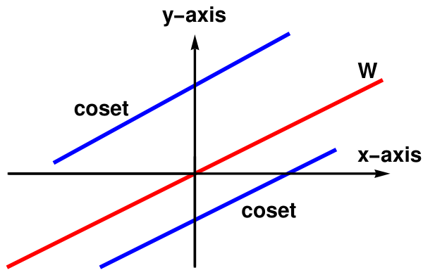
To see that all cosets are parallel lines, let us take point (𝑎, b) in ℝ² and notice that \[ \left[ (a, b) \right] = (a, b) + W = \left\{ (a, b) + (2t, t) \ : \ t \in \mathbb{R} \right\} . \] Thus, cosets (𝑎, b) + W can be identified with lines in the xy-plane given by y = ½x + (b − 𝑎). On the other hand, if ℓ is any line in ℝ² with slope ½, then ℓ is given by y = ½x + c, for some c in ℝ. In this case, we can write \[ \ell = \left\{ (2t, t) \ : \ t \in \mathbb{R} \right\} , \] allowing us to see ℓ as the coset (0, c) + W.
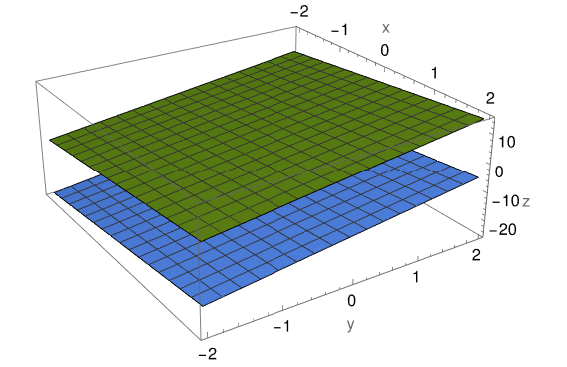
Similarly, if V = ℝ³ and W is a plane through the origin, its cosets are all of the parallel plane, and we can imagine this as filling up ℝ³ with a stack of planes.
Observation: If V is a vector space with subspace W, then W-cosets partition V.
Since 0 is in W, any v in V belongs to v + W. This proves that every v in V belongs to a W-coset and that each W-coset is nonempty.
That parts (a) and (e) of Lemma 1 are logically equivalent means precisely that the intersection of distinct W-cosets is empty.
Strictly speaking, 𝔏² functions are equivalence classes of functions that are equal almost everywhere (i.e., they differ on a set of Lebesgue measure zero). Let V = 𝔏²([0,1]), the space of square-integrable functions on [0,1], and let W be the subspace of functions that are zero almost everywhere. Then V/W is just 𝔏²([0,1]) as we usually define it: equivalence classes of functions that differ only on sets of measure zero 𝔏² functions can be understood as functions whose "energy" is finite, making them essential in areas like quantum mechanics and Fourier analysis.
The integral in definition of 𝔏² is unaffected by changes on sets of measure zero. To make 𝔏² a proper vector space and Hilbert space, we must identify functions that differ only on negligible sets. This avoid pathological behavior and ensures that operations like inner products and norms are well-defined.
Vector space addition and scalar multiplication are defined on equivalence classes. The corresponding dot product \[ f \bullet g = \int_0^1 f(x)\,g(x)\,{\text d}x \] is defined for equivalence classes. Then every Cauchy sequence has a limit in 𝔏² making it a Hilbert space. ■
Lemma 1: Let V be a vector space with subspace W. If v and x belong to V, then the following statements are logically equivalent:
- v is in x + W;
- v − x is in W;
- x − v is in W;
- x is in v + W;
- x + W = v + W.
-
(a) ⇒ (b)
If v belongs to to x + W, then there is w in W such that \[ \mathbf{v} = \mathbf{x} + \mathbf{w} . \] In this case, v − x = w. This proves that (a) implies (b).
-
(b) ⇒ (c)
Suppose next that x − v is in W. Since W is a subspace, \[ - \left( \mathbf{v} - \mathbf{x} \right) = \mathbf{x} - \mathbf{v} \] is in W, so (b) implies (c).
-
(c) ⇒ (d)
Suppose that x − v = w is in W. We then have \[ \mathbf{x} = \mathbf{v} + \mathbf{w} \in \left[ \mathbf{v} \right] = \mathbf{v} + W \] providing that (c) implies (d).
-
(d) ⇒ (e)
Suppose that x is in v + W with x = v + w₁ for w₁ in W. This means that for any w₂ in W, \[ \mathbf{x} + \mathbf{w}_2 = \mathbf{v} + \left( \mathbf{w}_1 + \mathbf{w}_2 \right) \in \mathbf{v} + W . \] This shows that (d) implies x + W ⊆ v + W. Switching the roles of v and x and then repeating the same argument, we get v + W ⊆ x + W. This is enough to prove that (d) implies (e).
-
(e) ⇒ (a)
Finally suppose x + W = v + W. This means that for each w₁ in W, there is w₂ in W so that \[ \mathbf{v} + \mathbf{w}_a = \mathbf{x} _+ \mathbf{w}_2 . \] We then have \[ \mathbf{v} = \mathbf{x} + \left( \mathbf{w}_2 - \mathbf{w}_1 \right) \in \mathbf{x} + W. \] This shows that (e) implies (a); Hence, all statements of the lemma logically equivalent.
- It is clear that x ∼ x because (x − x) = 0, which is an integer.
- If x ∼ y, then (x − y) is an integer. Its negation, (y − x) also belongs to ℤ because ℤ contains both, n and −n.
- We need to show that if x ∼ y and y ∼ z, then x ∼ z. Indeed, the latter holds if and only if (x − z) ∈ ℤ. By adding and subtracting y, we get \[ x - z = \left( x - y \right) + \left( y - z \right) . \] Since every term in parenthesis is an integer, their sun is also an integer. This proves transitivity of this relation.
Theorem 3: If V is a vector space with subspace W, then V/W is a vector space with addition defined by \[ ({\bf v}_1 + W ) + ({\bf v}_2 + W ) := ({\bf v}_1 + {\bf v}_2 ) + W \] and scaling defined by \[ k \left( {\bf v} + W \right) := k\,{\bf v} + W = \left[ k\,{\bf v} \right] . \]
Suppose vi + W = xi + W for vi and xi in V, i = 1, 2. Applying Lemma 1, we have vi − xi belonging to W. Since W is a subspace, \[ \mathbf{v}_1 - \mathbf{w}_1 + \mathbf{v}_2 - \mathbf{w}_2 = \left( \mathbf{v}_1 + \mathbf{v}_2 \right) - \left( \mathbf{x}_1 + \mathbf{x}_2 \right) \in W . \] It follows again by Lemma that \[ \mathbf{v}_1 + \mathbf{v}_2 + W = \mathbf{x}_1 + \mathbf{x}_2 + W , \] proving that addition is well-defined on V/W.
For scalar multiplication, we have to show that \[ \left[ k\,\mathbf{v} \right] = \left[ k\,\mathbf{u} \right] \qquad \Longrightarrow \qquad \mathbf{v} - \mathbf{u} \in W . \]
The Division Algorithm: Let n be a positive integer and let z be any other integer. Then there exists unique integers r and q such that
- z = q n + r,
- 0 ≤ r < n.
The subspace W = (2ℤ) of even integers is also subspace over field (2ℤ) itself.
Let ℤ₂ = ℤ/(2ℤ) be a quotient space, which is more appropriate to denote by GF(2). It stands for Galois Field, named after the brilliant mathematician Évariste Galois (1811--1832). It refers to a finite field—a set with a finite number of elements where you can perform addition, subtraction, multiplication, and division (except by zero), and all the usual field axioms hold.
ℤ₂ or GF₂ is the finite field with only two elements (0 and 1). GF(2) is the field with the smallest possible number of elements, and is unique if the additive identity and the multiplicative identity are denoted respectively 0 and 1, as usual. GF(2) can be identified with the field of the integers modulo 2, that is, the quotient ring of the ring of integers ℤ by the ideal 2ℤ of all even numbers: GF(2) = ℤ/(2ℤ).
In general, GF(p) is a Galois Field with p elements, where p is a prime number. Operations in GF(p) are done modulo p.
The multiplication of GF(2) is again the usual multiplication modulo 2 (see the table below), and on boolean variables corresponds to the logical AND (multiplication) operation and XOR (addition).
| + | 0 | 1 |
| 0 | 0 | 1 |
| 1 | 1 | 0 |
The multiplication of GF(2) is again the usual multiplication modulo 2 (see the table below), and on boolean variables corresponds to the logical AND operation.
| × | 0 | 1 |
| 0 | 0 | 0 |
| 1 | 0 | 1 |
You can also have fields of size pⁿ, where p is prime and n is a positive integer. These are extension fields and are crucial in coding theory, cryptography, and algebraic geometry. All fields of the same order are isomorphic, meaning they’re structurally identical even if represented differently. If you’re diving into error-correcting codes or cryptography algorithms, you’ll see GF(2⁸) pop up a lot—it’s the backbone of byte-level operations in things like AES encryption and Reed-Solomon codes. ■
The relation between the quotient space V/W. and subspaces of V that are complementary to W can now be stated as follows.
Theorem 4: Let W be a subspace of the vector space V, and let q be the quotient mapping of V onto V/W. Suppose U is a subspace of V. Then V = W ⊕ U if and only if the restriction of q to U is an isomorphism.
Also, q is injective on U; for suppose u₁ and u₂ are vectors in U and that qu₁ = qu₂. Then q(u₁ − u₂) = 0, so that u₁ − u₂ is in WThis vector is also in U, which is disjoint from W. Hence, u₁ − u₂ = 0. The restriction of q to U' is therefore a one-one linear transformation of U onto V/W.
Suppose U is a subspace of V such that q is one-one on U and q(U) = V/W. Let v be a vector in V. Then there is a vector u in U such that qu = qv, i.e., u + W = v + W. This means that v = w + u for some vector w in W. Therefore, V = W + U. To see that W and U are disjoint, suppose w is in both W and U. Since w is in W. we have qw = 0. However, q is one-to-one on U, and so it must be that w = 0. Thus, we have V = W ⊕ U.
Theorem 5: Let V be a finite-dimensional vector space over field 𝔽, W a subspace, and \[ \left\{ \mathbf{w}_1 , \ldots , \mathbf{w}_m \right\} , \quad \left\{ \mathbf{w}_1 , \ldots , \mathbf{w}_m , \mathbf{u}_1 , \ldots \mathbf{u}_{n-m} \right\} \] be ordered bases of W and V, respectively. Then image vectors {qu₁, … , qun-m} under canonical transformation \eqref{EqQuotient.1} form a basis in quotient space V/W.
Choose an element x ∈ V/W, and pick a representative v ∈ V of x (i.e., x = [v] = v + W ∈ V/W). Since {w₁, w₂, … , wm, u₁, … , un-m} spans V, we can write \[ \mathbf{v} = \sum_{i=1}^m a_i \mathbf{w}_i + \sum_{j=1}^{n-m} b_j \mathbf{u}_j . \] Applying the linear projection q : V ⇾ V/W to this linear combination, we get \[ \mathbf{x} = \left[ \mathbf{v} \right] = \sum_{i=1}^m a_i q\mathbf{w}_i + \sum_{j=1}^{n-m} b_j q\mathbf{u}_j = \sum_{j=1}^{n-m} b_j \left[ \mathbf{u}_j \right] \] because images of wi vanish for all i. Thus, images of uj span V/W.
To prove linear independence of vectors {q(u₁), &hellip , q(un-m)} = {[u₁], [u₂], … , [un-m]}, we assume that \[ \sum_{j=1}^{n-m} c_j \left[ \mathbf{u}_j \right] = 0 \] for some coefficients cj ∈ 𝔽. Then we need to show all these coefficients are zeroes. Let us consider the element \( \displaystyle \quad \mathbf{u} = \sum_{j=1}^{n-m} c_j \mathbf{u}_j \in V . \quad \) Its projection is zero in V/W. Then we conclude that vector u belongs to W, which leads to conclusion that u is spanned on vectors {w₁, w₂, … , wm}. So we get \[ \mathbf{u} = \sum_{j=1}^{n-m} c_j \mathbf{u}_j = \sum_{k=1}^m d_k \mathbf{w}_k , \] for some coefficients dk ∈ 𝔽. This can be rewritten as \[ V \ni \sum_{j=1}^{n-m} c_j \mathbf{u}_j + \sum_{k=1}^m \left( -d_k \right) \mathbf{w}_k = \mathbf{0} . \tag{E.1} \] By assumption, vectors {w₁, … , wm, u₁, … , un-m} form a basis in V, so they are linearly independent. Therefore, equation (E.1) holds only when all coefficients are zero. In particular, all coefficients cj are zeroes. and vectors {[u₁. *hellip; , [un-m]} are linear independent.
We consider two subspaces starting with the following one: \[ W = \left\{ \left( 1, 1, 1 \right) , \quad\left( 0, 0, 0 \right) \right\} . \] Since W = span{(1, 1, 1)}, it is one dimensional vector space.
There are four cosets modulo W: \begin{align*} \left[ \left( 1, 1, 1 \right) \right] &= W = \left\{ \left( 1, 1, 1 \right) \quad\left( 0, 0, 0 \right) \right\} , \\ \left[ \left( 1, 1, 0 \right) \right] &= \left\{ \left( 1, 1, 0 \right) \quad\left( 0, 0, 1 \right) \right\} , \\ \left[ \left( 1, 0, 1 \right) \right] &= \left\{ \left( 1, 0, 1 \right) \quad\left( 0, 1, 0 \right) \right\} , \\ \left[ \left( 0, 1, 1 \right) \right] &= \left\{ \left( 0, 1, 1 \right) \quad\left( 1, 0, 0 \right) \right\} . \end{align*} The quotient space is spanned on two of them: \[ V/W = \mbox{span} \left\{ \left[ \left( 1, 0, 1 \right) \right] , \quad \left[ \left( 1, 1, 0 \right) \right] \right\} . \] because two other coesets are linear combination of these two: \[ \left( 0, 1, 1 \right) = \left( 1, 0, 1 \right) + \left( 1, 1, 0 \right) . \] So we have \[ \dim \left( V/W \right) = \dim V - \dim W = 3 - 1 = 2 . \]
Now we consider two-dimensional subspace W: \[ W = \mbox{span} \left\{ \left( 1, 1, 1 \right) , \quad \left( 1, 1, 0 \right) \right\} . \] There are two cosets modulo W: \begin{align*} \left[ \left( 1, 1, 1 \right) \right] &= W = \left\{ \left( 1, 1, 1 \right) \quad\left( 0, 0, 0 \right) \quad \left( 1, 1, 0 \right) \quad \left( 0, 0, 1 \right) \right\} , \\ \left[ \left( 1, 0, 1 \right) \right] &= W = \left\{ \left( 1, 0, 1 \right) \quad\left( 0, 1, 0 \right) \quad \left( 0, 0, 0 \right) \quad \left( 1, 1, 1 \right) \right\} . \end{align*} Since the dimension of V/W is 1, we have \[ \dim \left( V/W \right) = \dim V - \dim W = 3 - 2 = 1 . \] ■
Corollary 1: Let V be a finite dimensional vector space with subspace, W. Then dim(V/W) = dim V - dim W.
Theorem 6: Let U be a subspace of a finite dimensional vector space V over a field 𝔽. Then dim(V/U) = dimV − dimU.
Theorem 6: Let V and U be vector spaces over the field 𝔽. Suppose T is a linear transformation of V onto U. If W is the null space of T, then U is isomorphic to V/W.
We can verify that ϕ is linear and sends V/W onto U because T is a linear transformation of V onto U.
The subgroup of rotations around a fixed axis—say, the z-axis is denoted by SO(2). It stabilizes a point on the sphere (e.g., the north pole). The dimension of the Special Orthogonal Group SO(2) is 1. The group SO(2) consists of 2 × 2 real orthogonal matrices with a determinant of 1. These matrices represent rotations in a 2-dimensional plane. A general element of SO(2) can be expressed as: \[ \begin{bmatrix} \cos\theta & -\sin\theta \\ \sin\theta & \phantom{-}\cos\theta \end{bmatrix} , \] where 𝜃 is the angle of rotation. Since the entire group is parameterized by a single variable, θ, the dimension of SO(2) is 1. This corresponds to the number of independent parameters required to specify an element of the group.
Let SO(3) act on sphere S² by rotating points. This action is:
- Transitive: Any point on the sphere can be rotated to any other point.
- Smooth: The action is differentiable.
The quotient space SO(3)/SO(2) consists of left cosets: \[ SO(3)/SO(2) = \left\{ g\, SO(2)\ \mid \ g \in SO(3) \right\} . \] Each coset corresponds to a unique point on the sphere. So we get a smooth bijection: \[ SO(3)/SO(2) \cong S^2 , \] This means the sphere ib ℝ³ can be viewed as the space of all rotations modulo those that fix a point—i.e., the orbit space of the action. According to Corollary 1, dim(SO(3)/SO(2)) = 3 −1 = 2.
Think of SO(3) as the full freedom of rotation. SO(2) is the “redundant” part—rotations that don’t move the chosen point. The quotient SO(3)/SO(2) captures the essential directions you can rotate to reach any point on the sphere. ■
Theorem 7: Every subspace of a vector space V is the kernel of a linear transformation on V.
Let M be a smooth manifold (it's a geometrical object that locally resembles Euclidean space, like a sphere or a torus) and p is a point in M. If you are not familiar with some mathematical tricks such as chart (local coordinate system), atlas, or germ, you may think about manifolds as geometrical objects embedded in ℝN, where N ≤ n + 1 is a positive integer.
The tangent space TpM is a vector space that captures the directions in which one can tangentially pass through p. It generalizes the idea of a tangent line to a curve or a tangent plane to a surface.There are several equivalent ways to define TpM:
- Via curves: A tangent vector at p is the velocity vector of a smooth curve γ(t) with γ(0) = p. \[ \mathbf{v}(f) = \left.\frac{\text d}{{\text d}t} f(\gamma(t)) \right|_{t=0} . \]
- Via derivative operators: A tangent vector is a linear map v: ℭ∞p(M) ↦ ℝ satisfying the Leibniz rule: \[ \mathbf{v}(fg) = \mathbf{v}(f)\,g(p) + f(p)\,\mathbf{v}(g) . \]
- Via coordinates: In a chart (or local coordinate map) (U, ϕ) around p, with coordinates (xⁱ, … , xn), every tangent vector can be written as: \[ \mathbf{v} = \sum_{i=1}^n v(x^i) \frac{\partial}{\partial x^i}\bigg|_p . \]
To make a rigorous definition of tangent vector, we need the following definition of equivalence classes:
Definition 1: Given a ℭk manifold, M, of dimension n, for any point p ∈ M, two ℭ¹-curves, γ₁ : (−ε₁, ε₁) ↦ M and γ₂ : (−ε₂, ε₂) ↦ M through p (i.e., γ₁(0) = γ₂(0) = p) are equivalent if and only if there is some chart (U, ϕ) at p so that \[ \left( \phi \circ \gamma_1 \right)' (0) = \left( \phi \circ \gamma_2 \right)' (0) . \] ▣
Now, the problem is that this definition seems to depend on the choice of the chart. Fortunately, this is not the case.
Definition 2: Given a ℭk manifold, M, of dimension n, with k ≥ 1, for any point p ∈ M, a tangent vector to M at p is any equivalence class of ℭ¹-curves through p on M modulo the equivalence relation defined in Definition 1. The set of all tangent vectors at p is denoted by TpM or Tp(M); this vector space of dimension n is called the tangent space. ▣
Observe that unless M = ℝn, in which case, for any p, q ∈ ℝn, the tangent space Tq(M) is naturally isomorphic to the tangent space Tp(M) by the translation q − p, for an arbitrary manifold, there is no relationship between Tp(M) and Tq(M) when p ≠ q.
One drawback of the definition of a tangent vector via curves is that it has no clear relation to the ℭk-differential structure of M. In particular, the definition does not seem to have anything to do with the functions defined locally at p. Other way two definitions of tangent vectors reveal this connection more clearly, but we do not purdue these options because it will require heavy mathematical techniques,
Now we consider a practical case when the manifold is embedded into ℝN. Let U ⊂ ℝn be an open set in finite dimensional space. The tangent space of U is the set of pairs (p, v) ∈ U × ℝn. When point p is identified with the vector started from the origin, then vector v must be orthogonal to this vector.
Let us consider a torus in ℝ³---it is a smooth 2-dimensional surface in ℝ³, like the surface of a donut. A torus can be described by a parametric equation, like \begin{align*} x &= \left( R + r\, \sin\theta \right) \cos\varphi , \\ y &= \left( R + r\, \sin\theta \right) \sin\varphi , \\ z &= r \, \cos\theta , \end{align*} where θ, φ are angular coordinates (parameters) and R and r are the major and minor radii respectively, or by an implicit Cartesian equation, which for a torus centered at the origin with its hole around the z-axis, is \[ \left( \sqrt{x² + y²} - R \right)^2 + z^2 = r^2 . \]
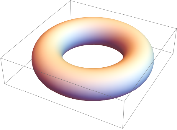
The tangent space of a torus embedded in ℝ³ is a 2-dimensional vector space that "touches" the torus at a single point and contains all possible directions in which you can tangentially pass through that point on the surface. At any point p on the torus, the tangent space TpT² is a plane that:
- Is tangent to the surface at p.
- Lies entirely within ℝ³.
- Is perpendicular to the normal vector at p.
Since the torus is a smooth manifold modeled on ℝ² / ℤ², its tangent space at any point p ∈ T² is naturally isomorphic to: \[ T_pT^2 \cong \mathbb{R}^2 \] Why? Because the action of ℤ² on ℝ² is by translations, which are smooth and free — so the quotient inherits a smooth structure, and the tangent space at any point is just the tangent space of ℝ² modulo the identification.
More Formally.
Let π : ℝ² ↦ T² be the quotient map. Then for any point p = π(x), the tangent space is:
\[
T_pT^2 = T_x\mathbb{R}^2 / T_x\mathbb{Z}^2 .
\]
However, since ℤ² is discrete, its tangent space is trivial, so:
\[
T_pT^2 \cong T_x\mathbb{R}^2 \cong \mathbb{R}^2 .
\]
The torus T² = ℝ² / ℤ² is not just a quotient space — it's also a Lie group.
The group operation is inherited from vector addition on ℝ².
Since ℤ² acts by translations, the quotient inherits a smooth group structure.
So T² becomes a compact, abelian Lie group of dimension 2.
■
Let V be a finite dimensional vector space over field 𝔽 and W ⊆ V a subspace. Unfortunately, there is no universal notation for dual spaces, some authors use prime,, others prefer asterisk. We will use the latter and denote by V ′ the dual space (the set of all linear forms/functional on the vector space) of V.
The dual of the quotient space (V/W) ′ is naturally isomorphic to the subspace of the dual space that vanishes on W. The later is denoted as W⁰ = {ψ ∈ V ′ : ψ(w) = 0, ∀ w ∈ W}, the annihilator of W. A beautiful relationship between these vector spaces is formulated in the following statement.
Theorem 8: Let V be a vector space over a field 𝔽 and W be a subspace of V. Then \[ W' \cong V' / W^0 , \] where W⁰ is the annihilator of W.
Now we show that f is onto. Then we show that any given χ ∈ W⁰ is the restriction of some φ ∈ W⁰. Let { w₁, w₂, … , wm } be a basis of W. Then it can be extended to a basis of V, say { w₁, w₂, … , wm, u₁, u₂, … , ur }, where m + r = dimV. Hence, we can write V = W ⊕ U, where U is a subspace of V spanned by { u₁, u₂, … , ur }. Now for any χ ∈ W✶ define ξ ∈ V✶ such that for any v ∈ V, v = w + v and ξ(v) = χ(w), where w ∈ W, u ∈ U. Let v₁ = v₂ and suppose that v₁ = w₁ + u₁ and v₂ = w₂ + u₂, where w₁, w₂ ∈ W and u₁, u₂ ∈ u. This implies that w₁ = w₂ and u₁ = u₂. As χ is a linear map, we get χ(w₁) = χ(w₂). This implies that ξ(v₁) = ξ(v₂) so ξ is well defined. It can be seen that ξ is a linear functional whose restriction on W is χ, i.e., f(ξ) = ξ|W = χ. Hence, f is onto and by fundamental theorem of vector space homomorphism W✶ ≌ V✶/Ker(f), namely, W✶ ≌ V✶/W⁰.
- V/W ≌ ℝ².
- V′ ≌ ℝ³ (dual space of linear functionals).
- The annihilator W⁰ ⊂ V′ consists of all linear forms ψ such that ψ(0, 0, 1) = 0.
- So (V/W)′ ≌ W⁰ ≌ span{(1, 0, 0), (0, 1, 0)}.
Solvability
Conversely, let kerf ⊂ kerg. We first construct h on the subspace imf ⊂ U. The only possibility is to set h(y) = g(x) if y = f(x). It is necessary to verify that h is determined uniquely and linearly on im(f). The first property follows from the fact that if y = f(x₁) = f(x₂), then x₁ − x₂ ∈ ker(f) ⊂ ker(g), whence g(x₁) = g(x₂). The second property follows automatically from the linearity of f and g.
Now it is sufficient to extend the mapping h from the subspace im(f) ⊂ U into the entire space U, for example, by selecting a basis in im(f), extending it up to a basis in U, and setting h equal to zero on the additional vectors.
- For each vector b in V there is a vector x in V so that T(x) = b and then the equation T(x) = 0 has only zero solutions. In other words: T is surjective (and so also bijective, since V is finite-dimensional).
- dim(ker(T)) > 0, so this equation cannot be solved for all b ∈ V and then the homogeneous equation T(x) = 0 as non-zero solutions.
If the index is positive, the operator's kernel is non-trivial, meaning it has infinitely many solutions for b in its image. The operator T is not injective (one-to-one), so the equation T(x) = b is only solvable if b is in the image of T. There may be some b for which T(x) = b has no solution. However, when a solution does exist, there are infinitely many solutions, because ker(T) has positive dimension. The solution set is an affine space modeled on ker(T).
If index is negative (dim(X) < dim(Y)), then the operator T is not surjective (onto), so its image is a proper subspace of Y, so there exist vectors b ∈ Y that are not in the image of T. The equation T(x) = b is only solvable if b is in the image of T. If solution exists, it may be unique.
In essence, for finite-dimensional operators, a zero index guarantees solvability for any b. A non-zero index means the operator is not surjective and thus not always solvable.
-
This exercise shows that every nonempty set has at least two partitions.
Let X be a nonempty set. Prove the following.
- {X} is a partition of X with single class (every element of X is inhabitant of this single class);
- { {x} : x ∈ X } is a partition of X with inifinitely many rooms, one for each element of X (recall that {𝑥} is not the same as 𝑥!).
-
For each of the following statements, find a partition of ℕ = {0, 1, 2, …} satisfying the
stated requirement. You will create different partitions for each of the requirements.
- Every room of the partition has exactly two inhabitants.
- There are exactly three rooms in the partition.
- There are infinitely many rooms in the partition, and each room has infinitely many inhabitants.
- Define the relation ∼ on ℝ by declaring 𝑥 ∼ 𝑦 if and only if 𝑥 − 𝑦 = 2𝜋𝑘 for some 𝑘 ∈ ℤ. Sjow that ∼ is an equivalence relation.
- Let ℭ[0, 1] be the set of all continuous real-valued functions on the interval [0, 1] ⊂ ℝ. For 𝑓, 𝑔 ∈ ℭ[0, 1], define 𝑓 ∼ 𝑔 if and only if \[ \int_0^1 f(x)\,{\text d}x = \int_0^1 g(x)\,{\text d}x . \] Show that ∼ is an equivalence relation and determine its equivalence classes.
- Let R be a relation defined on &Ropf'² by \[ \left( a, b \right) \ R \ \left( c, d \right) \qquad \iff \qquad a+d = b+c . \] Show that R is
- Axier, S., Linear Algebra Done Right. Undergraduate Texts in Mathematics (3rd ed.). Springer. 2015, ISBN 978-3-319-11079-0.
- Beezer, R.A., A First Course in Linear Algebra, 2017.
- Dillon, M., Linear Algebra, Vector Spaces, and Linear Transformations, American Mathematical Society, Providence, RI, 2023.
- Halmos, Paul Richard (1974) [1958]. Finite-Dimensional Vector Spaces. Undergraduate Texts in Mathematics (2nd ed.). Springer. ISBN 0-387-90093-4.
- Roman, Steven (2005). Advanced Linear Algebra. Undergraduate Texts in Mathematics (2nd ed.). Springer. ISBN 0-387-24766-1.