The position and orientation of an object in real life can be described with direction and magnitude e.g., eclipse is observed by many people from different locations. Information about an object (eclipse in our case) is given in the context of a reference frame. For example, in computer graphics objects need to be expressed with respect to the camera frame. Transformation of coordinates (position and orientation) from one frame of reference into another one is a fundamental operation in several areas: flight control of aircraft and rockets, movement of manipulators in robotics, and computer graphics.

In many applications, a problem described using one coordinate system may be solved more easily by switching to a new coordinate system. This switch is usually accomplished by performing a change of variables, a process that you have probably encountered in other mathematics courses. In linear algebra, a basis provides us with a coordinate system for a vector space, via the notion of coordinate vectors. Choosing the right basis will often greatly simplify a particular problem.


Change of basis

We start with some motivated examples for changing bases in ℝ², where illustration provides an additional insight to this topic.
Example 3: Show that the set of three polynomials β = {x + x², 2 + x, 3 + x²} forms a basis for ℝ≤2[x]

Solution: First, we show that these three polynomials are linearly independent. So we consider their linear combination and equate it to zero: \[ c_1 \left( x + x^2 \right) + c_2 \left( 2 + x \right) + c_3 \left( 3 + x^2 \right) = 0. \] The collecting similar terms, we get \[ 2\, c_2 + 3\, c_3 + \left( c_1 + c_2 \right) x + \left( c_1 + c_3 \right) x^2 = 0 . \] A polynomial is equal to zero only when all its coefficients are zeroes. So we get a system of equations \[ \begin{split} 2\,c_2 + 3\,c_3 &= 0 , \\ c_1 + c_2 &= 0, \\ c_1 + c_3 &= 0. \end{split} \] This system has only trivial solution c₁ = c₂ = c₃ = 0. Therefore, the given set of polynomials is a linear independent.

End of Example 3


Example 7: For any nonzero vector u in ℝ³, we consider the linear transformation
\[ T({\bf x}) = {\bf x} \times {\bf u} , \]
where × is the cross product operation. or standard basis in the Cartesian space ℝ³, we have
\[ T({\bf x}) = {\bf x} \times {\bf u} = \begin{pmatrix} x_1 \\ x_2 \\ x_3 \end{pmatrix} \times \begin{pmatrix} u_1 \\ u_2 \\ u_3 \end{pmatrix} = \begin{pmatrix} x_2 u_3 - x_3 u_2 \\ x_3 u_1 - x_1 u_3 \\ x_1 u_2 - x_2 u_1 \end{pmatrix} . \]
Therefore, when we use column vectors from ℝ3×1, transformation T can be written as a matrix multiplication
\[ T({\bf x}) = {\bf x} \times {\bf u} = {\bf A}\,{\bf x} , \]
where
\[ \left[ T \right] = {\bf A} = \begin{bmatrix} 0 & u_3 & -u_2 \\ -u_3 & 0 & u_1 \\ u_2 & -u_1 & 0 \end{bmatrix} . \]
This singular matrix A has one real eigenvalue λ₁ = 0 and two pure imaginary eigenvalues
\[ \lambda_1 = 0, \qquad \lambda_{2,3} = \pm {\bf j} \sqrt{u_1^2 + u_2^2 + u_3^2} = \pm {\bf j}\,\| {\bf u} \| . . \]
A = {{0, u3, -u2}, {-u3, 0, u1}, {u2, -u1, 0}} Eigenvalues[A]
{0, -Sqrt[-u1^2 - u2^2 - u3^2], Sqrt[-u1^2 - u2^2 - u3^2]}
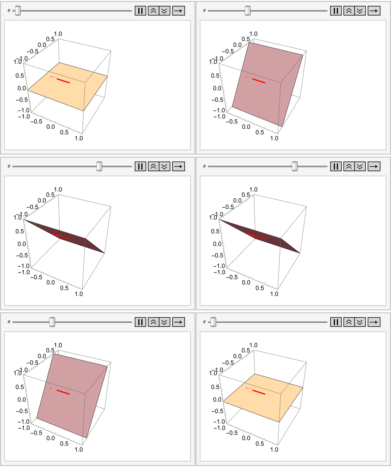
The null space of T is the line through the origin spanned by vector u and its image is the plane through the origin orthogonal to u.

However, we may still be able to find a basis for ℝ³ more suitable than standard for the purposes of representing our transformation T. Let us exploit the fact that ker(T) and im(T) are orthogonal subspaces. Consider, for instance, the following choice of orthogonal basis

\[ \alpha = \left\{ {\bf w}_1 = \begin{bmatrix} u_1 \\ u_2 \\ u_3 \end{bmatrix} , \quad {\bf w}_2 = \begin{bmatrix} u_3 \\ 0 \\ -u_1 \end{bmatrix} , \quad {\bf w}_3 = \begin{bmatrix} u_2 \\ - u_1 \\ 0 \end{bmatrix} \right\} . \]
We can check that vectors w₂ and w₃ are orthogonal to w₁. Of course, Mathematica is happy to assist you.
Dot[{u1, u2, u3}, {u3, 0, -u1}]
0
Dot[{u1, u2, u3}, {u2, -u1, 0}]
0
Moreover, these vectors are linearly independent because the determinant of these three vectors is not zero. Hence, α is a basis.
Det[{{u1, u2, u3}, {u3, 0, -u1}, {u2, -u1, 0}}]
-u1^3 - u1 u2^2 - u1 u3^2
Since u = w₁, we have \begin{align*} T( {\bf w}_1 ) &= {\bf w}_1 \times {\bf w}_1 = {\bf 0} , \\ T( {\bf w}_2 ) &= {\bf w}_2 \times {\bf w}_1 = {\bf A}\,{\bf w}_2 = \begin{pmatrix} u_3 \\ 0 \\ -u_1 \end{pmatrix} \times \begin{pmatrix} u_1 \\ u_2 \\ u_3 \end{pmatrix} = \begin{pmatrix} u_1 u_2 \\ - u_1^2 - u_3^2 \\ u_2 u_3 \end{pmatrix} \\ &= 0 {\bf w}_1 - \frac{u_2 u_3}{u_1}\, {\bf w}_2 + \left( u_1 + \frac{u_3^2}{u_1} \right) {\bf w}_3 , \\ T( {\bf w}_3 ) &= {\bf w}_3 \times {\bf w}_1 = {\bf A}\,{\bf w}_3 = \begin{pmatrix} u_2 \\ -u_1 \\ 0 \end{pmatrix} \times \begin{pmatrix} u_1 \\ u_2 \\ u_3 \end{pmatrix} = \begin{pmatrix} - u_1 u_3 \\ -u_2 u_3 \\ u_1^2 + u_2^2 \end{pmatrix} \\ &= 0 {\bf w}_1 - \left( u_1 + \frac{u_2^2}{u_1} \right) {\bf w}_2 + \frac{u_2 u_3}{u_1}\, {\bf w}_3 , \qquad\quad u_1 \ne 0. \end{align*}
A = {{0, u3, -u2}, {-u3, 0, u1}, {u2, -u1, 0}};
A . {u3, 0, -u1}
Cross[{u3, 0, -u1}, {u1, u2, u3}]
{u1 u2, -u1^2 - u3^2, u2 u3}
A . {u2, -u1, 0}
{-u1 u3, -u2 u3, u1^2 + u2^2}
Then transformation T in basis α is represented by the matrix, which we denote by B:
\[ \left[ T \right]_{\alpha} = {\bf B} = \begin{bmatrix} 0 & 0 & 0 \\ 0 & - \frac{u_2 u_3}{u_1} & - u_1 - \frac{u_2^2}{u_1} \\ 0 & u_1 + \frac{u_3^2}{u_1} & \frac{u_2 u_3}{u_1} \end{bmatrix} . \]
The eigenvalues of matrix B are the same as A (Mathematica confirms).
B = {{0, 0, 0}, {0, -u2*u3/u1, -u1 - u2^2 /u1}, {0, u1 + u3^2 /u1 , u2*u3/u1}};
Eigenvalues[B]
{0, -I Sqrt[u1^2 + u2^2 + u3^2], I Sqrt[u1^2 + u2^2 + u3^2]}
Moreover, these two matrices are similar, so there exists a non singular matrix S su ch that B = S−1AS.

In many respects, B is simpler than A, but it lacks skew-symmetry. Perhaps, a better choice would be to make w₂ and w₃ an orthogonal basis for im(A. Consider another basis

\[ \beta = \left\{ {\bf v}_1 = \begin{bmatrix} u_1 \\ u_2 \\ u_3 \end{bmatrix} , \quad {\bf v}_2 = \begin{bmatrix} u_3 \\ 0 \\ -u_1 \end{bmatrix} , \quad {\bf v}_3 = {\bf v}_2 \times {\bf v}_1 = \begin{bmatrix} u_1 u_2 \\ -u_3^2 - u_1^2 \\ u_2 u_3 \end{bmatrix} \right\} . \]
Cross[{u3, 0, u1}, {u1, u2, u3}]
{u1 u2, -u1^2 - u3^2, u2 u3}
In this new borthogonal basis β, matrix A is
\[ \left[ T \right]_{\beta} = {\bf C} = \begin{bmatrix} 0&0&0 \\ 0 & 0 & - \| {\bf u} \|^2 \\ 0 & 1 & 0 \end{bmatrix} , \]
because \begin{align*} T( {\bf v}_1 ) &= {\bf v}_1 \times {\bf v}_1 = {\bf 0} , \\ T( {\bf v}_2 ) &= {\bf v}_2 \times {\bf v}_1 = {\bf A}\,{\bf v}_2 = \begin{pmatrix} u_3 \\ 0 \\ -u_1 \end{pmatrix} \times \begin{pmatrix} u_1 \\ u_2 \\ u_3 \end{pmatrix} = \begin{pmatrix} u_1 u_2 \\ - u_1^2 - u_3^2 \\ u_2 u_3 \end{pmatrix} \\ &= 0\ {\bf v}_1 + 0 {\bf v}_2 + 1 \cdot {\bf v}_3 , \\ T( {\bf v}_3 ) &= {\bf v}_3 \times {\bf v}_1 = {\bf A}\,{\bf v}_3 = \begin{pmatrix} u_1 u_2 \\ -u_3^2 - u_1^2 \\ u_2 u_3 \end{pmatrix} \times \begin{pmatrix} u_1 \\ u_2 \\ u_3 \end{pmatrix} = \begin{pmatrix} - u_3 \left( u_3^2 + u_2^2 + u_1^2 \right) \\ 0 \\ u_1 \left( u_1^2 + u_2^2 + u_3^2 \right) \end{pmatrix} \\ &= 0\, {\bf v}_1 - \| {\bf u} \|^2 {\bf v}_2 + 0\, {\bf w}_3 , \qquad\quad u_1 \ne 0. \end{align*}
w3 = Cross[w2, w1] Cross[w3, w1]
{u1 u2, -u1^2 - u3^2, u2 u3}
A . w3
{-u2^2 u3 + u3 (-u1^2 - u3^2), 0, u1 u2^2 - u1 (-u1^2 - u3^2)}
Although matrix C is not skew symmetric, we can can adjust the lengths of vectors to obtain orthonormal basis for ℝ³:
\[ \beta_0 = \left\{ {\bf v}_1 = \frac{1}{\| {\bf u} \|} \begin{bmatrix} u_1 \\ u_2 \\ u_3 \end{bmatrix} , \quad {\bf v}_2 = \frac{1}{\sqrt{u_1^2 + u_3^2}} \begin{bmatrix} u_3 \\ 0 \\ -u_1 \end{bmatrix} , \quad {\bf v}_3 = \frac{1}{\| {\bf v}_3 \|} \,{\bf v}_2 \times {\bf v}_1 = \frac{1}{\| {\bf v}_3 \|} \,\begin{bmatrix} u_1 u_2 \\ -u_3^2 - u_1^2 \\ u_2 u_3 \end{bmatrix} \right\} . \]
Linear transformation T has the following matrix in basis β0
\[ \left[ T \right]_{\beta_0} = {\bf C}_0 = \begin{bmatrix} 0&0&0 \\ 0 & 0 & - \| {\bf u} \| \\ 0 & \| {\bf u} \| & 0 \end{bmatrix} . \]
The skew-symmetry is restored.he skew-symmetry is restored. The action of >i>T can be read off this matrix. Given any x = cu₁ + cu₂ + cu₃, T eliminates its u₁-component (orthogonal projection onto the uu₃-plane), stretches the uu₃-component by a factor of ∥v∥ (force magnitude) and rotates the result by an angle of 90° about the u₁-axis (clockwise). In the language of physics/mechanics, T gives the torque.

Since the basis β0 is orthonormal, matrix A is similar to C0. There exists an orthogonal matrix S such that \[ {\bf A} = {\bf S} \, {\bf C}_0 {\bf S}^{\mathrm T} . \]

End of Example 7


  1. Anton, Howard (2005), Elementary Linear Algebra (Applications Version) (9th ed.), Wiley International
  2. Beezer, R.A., A First Course in Linear Algebra, 2017.
  3. Fitzpatrick, S., Linear Algebra: A second course, featuring proofs and Python. 2023.