
Introduction to Linear Algebra
Systems of Linear Equations
- Introduction
- Linear systems
- Vectors
- Linear combinations
- Matrices
- Planes in ℝ³
- Equation A x = b
- Sensitivity of solutions
- Linear independence
- Plane transformations
- Space transformations
- Linear transformations
- Affine maps
- Exercises
- Answers
Matrix Algebra
- Introduction
- Manipulation of matrices
- Partitioned matrices
- Block matrices
- Matrix operators
- Determinants
- Cofactors
- Cramer's rule
- Chiò's method
- Equivalent matrices
- Elimination: A = L U
- PLU factorization
- Reflection
- Givens rotation
- Special matrices
- Exercises
- Answers
Vector Spaces
- Introduction
- Motivation
- Vector spaces
- Bases
- Dimension
- Coordinate systems
- Linear transformations
- Change of basis
- Matrix transformations
- Compositions
- Isomorphisms
- Dual transformations
- Quotient spaces
- Rank
- Solving A x = b
- Exercises
- Answers
Eigenvalues, Eigenvectors
- Introduction
- Characteristic polynomials
- Companion matrix
- Algebraic and geometric multiplicities
- Minimal polynomials
- Eigenspaces
- Where are eigenvalues?
- Eigenvalues of A B and B A
- Generalized eigenvectors
- Similarity
- Diagonalizability
- Self-adjoint operators
- Exercises
- Answers
Euclidean Spaces
- Introduction
- Euclidean space
- Bilinear transformations
- Norm and distance
- Matrix norms
- Dual norms
- Dual transformations
- Examples of transformations
- Orthogonality
- Gram--Schmidt Process
- Orthogonal matrices
- Self-adjoint matrices
- Unitary matrices
- Projection operators
- QR-decomposition
- Least Square Approximation
- Quadratic forms
- Exercises
- Answers
Canonical forms
- Introduction
- 2D decomposition
- 3D decomposition
- Projectors
- Direct-sum decompositions
- Cyclic decompositions
- Symmetric matrices
- Pseudoinverse
- URV-decomposition
- LU-decomposition
- QR-decomposition
- Cholesky decomposition
- Schur decomposition
- Positive matrices
- Roots
- Polar factorization
- Spectral decomposition
- CUR decomposition
- Exercises
- Answers
Applications
- Introduction
- TNB frames
- Introduction
- GPS problem
- Coriolis acceleration
- Poisson equation
- Graph theory
- Error correcting codes
- Electric circuits
- FSA
- Markov chains
- Cryptography
- Wave-length transfer matrix
- Computer graphics
- Linear Programming
- Hill's determinant
- Fibonacci matrices
- Discrete dynamic systems
- Discrete Fourier transform
- Fast Fourier transform
- Curve fitting
- Answers
Miscellany
- Introduction
- Circles along curves
- TNB frames
- Differential forms
- Calculus
- Vector representations
- Matrix representations
- Change of basis
- Orthonormal Diagonalization
- Generalized inverse
- Differential forms
Preliminaries
- Complex Number Operations
- Sets
- Polynomials
- Polynomials and Matrices
- Computer solves Systems of Linear Equations
- Location of Eigenvalues
- Power Method
- Iterative Method
- Similarity and Diagonalization
Glossary
Reference

This Book is licensed under Creative Commons Attribution-NonCommercial-NoDerivs 3.0 Unported License
This section is divided into a few of subsections, links to which are: Vector products
Triple Scalar Product
The triple scalar product of three noncoplanar vectors a = (𝑎₁, 𝑎₂, 𝑎₃), b = (b₁, b₂, b₃), and c = (c₁, c₂, c₃) written in Cartesian coordinates is
\begin{equation} \label{EqTriple.1}
{\bf a} \bullet {\bf b} \times {\bf c} = \det \begin{bmatrix} a_1 & a_2 & a_3 \\ b_1 & b_2 & b_3 \\ c_1 & c_2 & c_3 \end{bmatrix}
\end{equation}
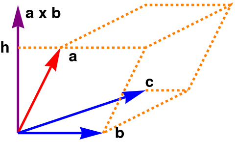
The scalar triple product of three vectors is the volume of parallelepiped spand on this three vectors:
\[
V = {\bf a} \bullet \left( {\bf b} \times {\bf c} \right) = h \left\vert {\bf b} \times {\bf c} \right\vert ,
\]
where h is the projection of a onto the direction of b × c.
a = Graphics[{Red, Thickness[0.01], Arrowheads[0.1],
Arrow[{{0, 0}, {0.5, 1}}]}];
b = Graphics[{Blue, Thickness[0.01], Arrowheads[0.1],
Arrow[{{0, 0}, {1, 0}}]}];
c = Graphics[{Blue, Thickness[0.01], Arrowheads[0.1],
Arrow[{{0, 0}, {1.5, 0.5}}]}];
bc = Graphics[{Purple, Thickness[0.01], Arrowheads[0.1],
Arrow[{{0, 0}, {0, 1.5}}]}];
line = Plot[1, {x, 0, 1.5},
PlotStyle -> {Thickness[0.01], Dashed, Orange}]\
l1 = Graphics[{Thickness[0.01], Dashed, Orange,
Line[{{1, 0}, {1.5, 1}, {2.5, 1.5}, {2, 0.5}, {1, 0}}]}];
l2 = Graphics[{Thickness[0.01], Dashed, Orange,
Line[{{1.5, 0.5}, {2, 0.5}}]}];
l3 = Graphics[{Thickness[0.01], Dashed, Orange,
Line[{{0.5, 1}, {1.5, 1.5}, {2.5, 1.5}}]}];
th = Graphics[
Text[Style["h", Bold, Black, FontSize -> 24], {-0.15, 1}]];
ta = Graphics[
Text[Style["a", Bold, Black, FontSize -> 24], {0.65, 0.9}]];
tb = Graphics[
Text[Style["b", Bold, Black, FontSize -> 24], {1.2, 0}]];
tc = Graphics[
Text[Style["c", Bold, Black, FontSize -> 24], {1.55, 0.6}]];
tab = Graphics[
Text[Style["a x b", Bold, Black, FontSize -> 24], {0.3, 1.4}]];
Show[bc, a, b, c, line, l1, l2, l3, th, ta, tb, tc, tab]
\[
{\bf a} \bullet \left( {\bf b} \times {\bf c} \right) = {\bf b} \bullet \left( {\bf c} \times {\bf a} \right) = {\bf c} \bullet \left( {\bf a} \times {\bf b} \right) .
\]
Hence, cyclicly permuting the vectors doesn’t change the value of the triple scalar product, which we denote as
\begin{equation} \label{EqTriple.2}
\begin{bmatrix} {\bf a} & {\bf b} & {\bf c} \end{bmatrix} = {\bf a} \bullet \left( {\bf b} \times {\bf c} \right) .
\end{equation}
Moreover, the scalar triple product vanishes if two of the vectors A, B and C
are identical (or parallel) :
\[
{\bf a} \bullet \left( {\bf b} \times {\bf a} \right) = {\bf b} \bullet \left( {\bf a} \times {\bf b} \right) = {\bf } \bullet \left( {\bf a} \times {\bf a} \right) = 0 .
\]
Three vectors a, b, and c are coplanar (linearly dependent) if and only if
they span a parallelepiped of zero volume, i.e. , if and only if their scalar triple product vanishes.
It follows that three vectors a, b, and c form a basis if
and only if a• (b × c) ≠ 0. The basis is said to be right-handed if a• (b × c) > 0
and left-handed if a• (b × c) < 0.
Example 1:
Let us consider three vectors (that we write as column vectors):
\[
{\bf a} = \left( 1, 2, 3 \right) , \quad {\bf b} = \left( -1 2, -4 \right) , \quad {\bf c} = \left( 3, 2, 1 \right) .
\]
First, we find cross product of vectors b and c:
\[
{\bf b} \times {\bf c} = \left( \right).
\]
Then the triple scalar product of these three vectors becomes
End of Example 1
■ Now we use the triple scalar product to define the reciprocal basis vectors. Suppose we are given non-Euclidean basis vectors
\[
{\bf e}_1 , \qquad {\bf e}_2 , \qquad {\bf e}_3 ,
\]
where e₁, e₂, e₃ are not necessarily of unit length. The corresponding basis system is sometimes called “covariant”, or “lowered”. The reciprocal (or dual or contracovariant) basis vectors are defined as
\begin{equation} \label{EqTriple.3}
{\bf e}^1 = \frac{{\bf e}_2 \times {\bf e}_3}{\left[ {\bf e}_1\,{\bf e}_2\,{\bf e}_3 \right]} , \quad {\bf e}^2 = \frac{{\bf e}_3 \times {\bf e}_1}{\left[ {\bf e}_1\,{\bf e}_2\,{\bf e}_3 \right]} , \quad {\bf e}^3 = \frac{{\bf e}_1 \times {\bf e}_2}{\left[ {\bf e}_1\,{\bf e}_2\,{\bf e}_3 \right]} .
\end{equation}
This reciprocal (raised) basis is orthonormal to the covariant (lowered) basis. We can easily verify this by dualing (which is actually dotting) one of the lowered basis vectors into its corresponding reciprocal. We find that
\[
\left\langle {\bf e}^3 , {\bf e}_2 \right\rangle =
{\bf e}^3 \bullet {\bf e}_2 = \frac{{\bf e}_1 \times {\bf e}_2}{\left[ {\bf e}_1\,{\bf e}_2\,{\bf e}_3 \right]} \bullet {\bf e}_2 = \frac{\left[ {\bf e}_2\,{\bf e}_1\,{\bf e}_2 \right]}{\left[ {\bf e}_1\,{\bf e}_2\,{\bf e}_3 \right]} = 0
\]
because of the corresponding property above showing that the triple scalar product of parallel vectors is 0.
Using this covariant basis, we can express any real numerical vector either as dual vector (so it becomes bra-vector) or as regular, covariant or ket-vector. We summarize properties of scalar triple products (which is denoted as [x y z]) in the following table.
| [u v w] = [v w u] = [w u v] = −[v u w] |
| [u u w] = [v u v] = 0 |
| [u v w]² = [(u × v) (v × w) (w × u)] |
| u [v w x] − v [w x u] + w [x u v] − x [u v w] = 0 |
| (u × v) × (w × x) = v [u w x] − u [v w x] |
| [(u × v) (w × x) (y × z)] = [v y z] [u w x] − [u w z] [v w x] |
| [(u + v) (v + w) (w + u)] = 2 [u v w] |
| \( \displaystyle \quad \begin{align*} \left[ ({\bf u} - {\bf x})\ ({\bf v} - {\bf x})\ ({\bf w} - {\bf x}) \right] &= \left[ {\bf u}\ {\bf v}\ {\bf w} \right] - \left[ {\bf u}\ {\bf v}\ {\bf x} \right] - \left[ {\bf u}\ {\bf x}\ {\bf w} \right] - \left[ {\bf x}\ {\bf v}\ {\bf w} \right] \\ &= \left[ ({\bf u} - {\bf x})\ {\bf v} \ {\bf w} \right] - \left[ ({\bf v} - {\bf w}) \ {\bf x} \ {\bf u} \right] \end{align*} \) |
| \( \displaystyle \quad \left[ {\bf u}\ {\bf v} \ {\bf w} \right] \ \left[ {\bf x}\ {\bf y} \ {\bf z} \right] =\begin{vmatrix} {\bf u} \bullet {\bf x} & {\bf u} \bullet {\bf y} & {\bf u} \bullet {\bf z} \\ {\bf v} \bullet {\bf x} & {\bf v} \bullet {\bf y} & {\bf v} \bullet {\bf z} \\ {\bf w} \bullet {\bf x} & {\bf w} \bullet {\bf y} & {\bf w} \bullet {\bf z} \\ \end{vmatrix}\) |
Example 2:
End of Example 2
■ Triple Vector Product
By the vector triple product of three vectors a, b, and c we mean the vector a × (b × c). Generally speaking, (a × b) × c ≠ a × (b × c). Clearly, a × (b × c) is perpendicular to a and lies in the plane of b and c.Suppose the vectors a, b, and c are noncollinear [otherwise a × (b × c)vanishes trivially]. Then a × (b × c) has a unique expansion of the form
\begin{equation} \label{EqTriple.4}
{\bf a} \times \left( {\bf b} \times {\bf c} \right) = \alpha\, {\bf b} + \beta\,{\bf c}
\end{equation}
for some scalars α and β ∈ ℝ.
To determine the scalars α and β, we introduce the vectors
\[
{\bf d} = {\bf b} \times {\bf c} = \left( d_1 , d_2 , d_3 \right) , \quad {\bf e} = {\bf a} \times \left( {\bf b} \times {\bf c} \right) = \left( e_1 , e_2 , e_3 \right) .
\]
Using definition of the cross product, we derive
\begin{align*}
e_1 &= a_2 d_3 - a_3 d_2 , \\
d_2 &= b_3 c_1 - b_1 c_3 , \\
d_3 &= b_1 c_2 - b_2 c_1 .
\end{align*}
It follows that
\begin{align*}
e_1 &= a_2 \left( b_1 c_2 - b_2 c_1 \right) - a_3 \left( b_3 c_1 b_1 c_3 \right)
\end{align*}
Adding and subtracting 𝑎₁b₁c₁ from the right-hand side and using definition of the dot product,
we find that
\begin{align*}
e_1 &= b_1 \left( a_1 c_1 + a_2 c_2 + a_3 c_3 \right) - c_1 \left( a_1 b_1 + a_2 b_2 + a_3 b_3 \right)
\\
&= b_1 \left( {\bf a} \bullet {\bf c} \right) - c_1 \left( {\bf a} \bullet {\bf c} \right) .
\end{align*}
In just the same way, it turns out that
\begin{align*}
e_2 &= b_2 \left( {\bf a} \bullet {\bf c} \right) - c_2 \left( {\bf a} \bullet {\bf c} \right) ,
\\
e_3 &= b_3 \left( {\bf a} \bullet {\bf c} \right) - c_3 \left( {\bf a} \bullet {\bf c} \right) .
\end{align*}
Therefore the coefficients α and β in Eq.\eqref{EqTriple.4} are
\[
\alpha = {\bf a} \bullet {\bf c} , \quad \beta = {\bf a} \bullet {\bf b} .
\]
Finally, we get
\begin{equation} \label{EqTriple.5}
{\bf a} \times \left( {\bf b} \times {\bf c} \right) = {\bf b} \left( {\bf a} \bullet {\bf c} \right) - {\bf c} \left( {\bf a} \bullet {\bf b} \right) .
\end{equation}
In a similar way, it can be shown that
\begin{equation} \label{EqTriple.6}
\left( {\bf a} \times {\bf b} \right) \times {\bf c} = {\bf b} \left( {\bf a} \bullet {\bf c} \right) - {\bf a} \left( {\bf b} \bullet {\bf c} \right) .
\end{equation}
Example 3:
Let us consider three vectors
\[
{\bf a} = \left( 1, 2, 3 \right) , \quad {\bf b} = \left( 2, -1, 1 \right) , \quad {\bf c} = \left( 3, 2, 1 \right) .
\]
Calculations show that
Cross[{1, 2, 3}, {2, -1, 1}]
{5, 5, -5}
\[
{\bf a} \times {\bf b} = \left( 5, 5, -5 \right) .
\]
Cross[{2, -1, 1}, {3, 2, 1}]
{-3, 1, 7}
\[
{\bf b} \times {\bf c} = \left( -3, 1, 7 \right) .
\]
Cross[Cross[{1, 2, 3}, {2, -1, 1}], {3, 2, 1}]
{15, -20, -5}
Cross[{1, 2, 3}, Cross[{2, -1, 1}, {3, 2, 1}]]
{11, -16, 7}
So we see that for these three vectors, we have
\[
{\bf a} \times \left( {\bf b} \times {\bf c} \right) = \left( 11, -16, 7 \right) \ne \left( 15, -20, -5 \right) = \left( {\bf a} \times {\bf b} \right) \times {\bf c} .
\]
Now we verify formulas (3) and (4). First, we calculate dot products:
\begin{align*}
{\bf a} \bullet {\bf b} &= 3 ,
\\
{\bf a} \bullet {\bf c} &= 10,
\\
{\bf b} \bullet {\bf c} &= 5 .
\end{align*}
{1, 2, 3} . {2, -1, 1}
3
{1, 2, 3} . {3, 2, 1}
10
and
{3, 2, 1} . {2, -1, 1}
5
Then we calculate
\[
{\bf a} \times \left( {\bf b} \times {\bf c} \right) = {\bf b} \left( {\bf a} \bullet {\bf c} \right) - {\bf c} \left( {\bf a} \bullet {\bf b} \right) = \left( 11, -16, 7 \right) .
\]
10*{2, -1, 1} - 3*{3, 2, 1}
{11, -16, 7}
and
\[
\left( {\bf a} \times {\bf b} \right) \times {\bf c} = {\bf b} \left( {\bf a} \bullet {\bf c} \right) - {\bf a} \left( {\bf b} \bullet {\bf c} \right) = \left( 15, -20, -5 \right) .
\]
10*{2, -1, 1} - 5*{1, 2, 3}
{15, -20, -5}
End of Example 3
■
- Mecholsky, N., Primer on the Basics of Tensor Analysis and the Laplacian in Generalized Coordinates, 2004.