Introduction to Linear Algebra
Systems of Linear Equations
- Introduction
- Linear systems
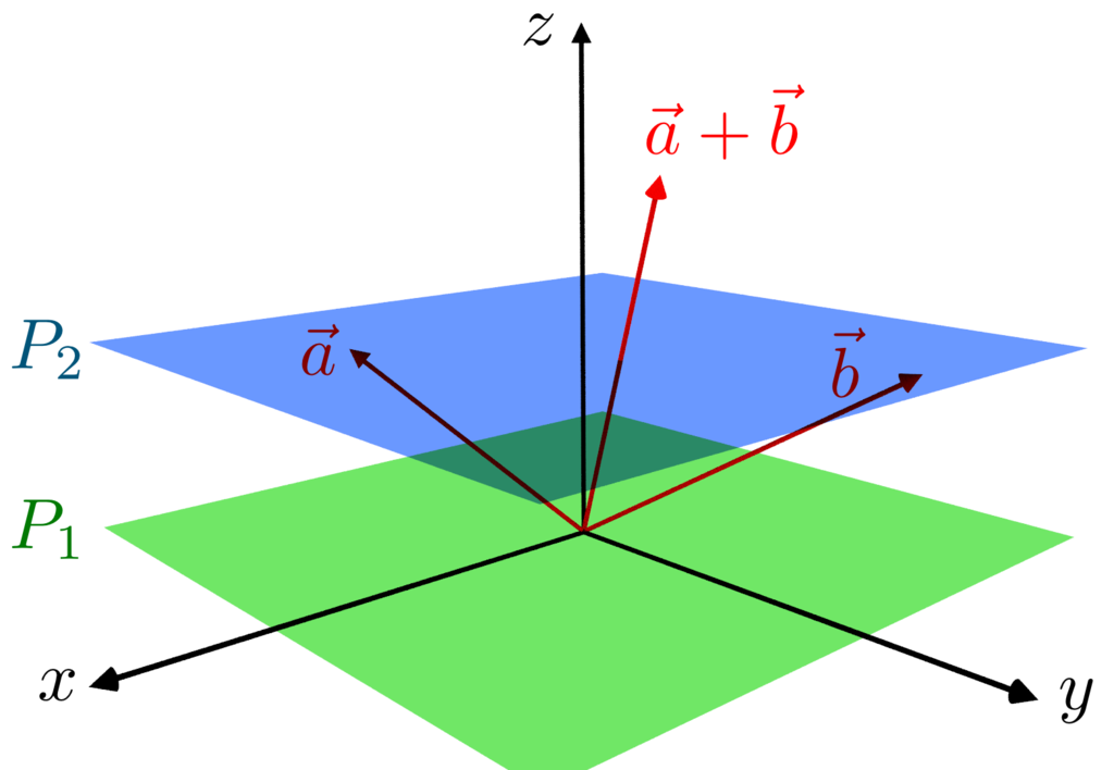
- Vectors
- Linear combinations
- Matrices
- Planes in ℝ³
- Reduced Row-Echelon Form
- Equation A x = b
- Sensitivity of solutions
- Linear independence
- Plane transformations
- Space transformations
- Linear transformations
- Affine maps
- Exercises
- Answers
Matrix Algebra
- Introduction
- Manipulation of matrices
- Partitioned matrices
- Block matrices Matrix operators
- Determinants
- Cofactors
- Cramer's rule
- Equivalent matrices
- Elimination: A = L U
- PLU factorization
- Reflection
- Givens rotation
- Special matrices
- Exercises
- Answers
Vector Spaces
- Introduction
- Motivation
- Vector spaces
- Bases
- Dimension
- Coordinate systems
- Linear transformations
- Change of basis
- Matrix transformations
- Compositions
- Isomorphisms
- Dual transformations
- Direct sums
- Quotient spaces
- Vector products
- Cross products
- Rank
- Solving A x = b
- Exercises
- Answers
Eigenvalues, Eigenvectors
- Introduction
- Characteristic polynomials
- Companion matrix
- Algebraic and geometric multiplicities
- Minimal polynomials
- Eigenspaces
- Where are eigenvalues?
- Eigenvalues of A B and B A
- Generalized eigenvectors
- Similarity
- Diagonalizability
- Self-adjoint operators
Euclidean Spaces
- Introduction
- Dot product
- Bilinear transformations
- Inner product
- Norm and distance
- Matrix norms
- Dual norms
- Dual transformations
- Examples of transformations
- Orthogonality
- Gram--Schmidt Process
- Orthogonal sets
- Self-adjoint Matrices
- Unitary matrices
- Projection operators
- QR-decomposition
- Least Square Approximation
- Quadratic forms
- Exercises
- Answers
Matrix Decompositions
- Introduction
- Symmetric matrices
- LU-decomposition
- QR-decomposition
- Cholesky decomposition
- Schur decomposition
- Positive matrices
- Roots
- Polar factorization
- Spectral decomposition
- Singular values
- SVD <
- Pseudoinverse
- Exercises
- Answers
Applications
- Introduction
- GPS problem
- Poisson equation
- Graph theory
- Error correcting codes
- Electric circuits
- Markov chains
- Cryptography
- Wave-length transfer matrix
- Computer graphics
- Linear Programming
- Hill's determinant
- Fibonacci matrices
- Discrete dynamic systems
- Discrete Fourier transform
- Fast Fourier transform
- Curve fitting
Functions of Matrices
- Introduction
- Diagonalization
- Sylvester formula
- The Resolvent method
- Polynomial interpolation
- Positive matrices
- Roots <
- Pseudoinverse
- Exercises
- Answers
Miscellany
- Introduction
- Circles along curves
- TNB frames
- Tensors
- Tensors in ℝ³
- Tensors & Mechanics
- Differential forms
- Calculus
- Vector representations
- Matrix representations
- Change of basis
- Orthonormal Diagonalization
- Generalized inverse
- Differential forms
Preliminaries
- Complex Number Operations
- Sets
- Polynomials
- Polynomials and Matrices
- Computer solves Systems of Linear Equations
- Location of Eigenvalues
- Power Method
- Iterative Method
- Similarity and Diagonalization
Glossary
Reference

This Book is licensed under Creative Commons Attribution-NonCommercial-NoDerivs 3.0 Unported License
https://math.mit.edu/~gs/linearalgebra/ila5/linearalgebra5_10-6.pdf
Computer Graphics
Computer graphics deals with images, stationary or that are moved around. Their scale is changed. Three dimensions are projected onto two dimensions. All the main operations are done by matrices—but the shape of these matrices is surprising. In Computer Graphics, matrices are used to represent many different types of data. Games that involve 2D or 3D graphics rely on some matrix operations to display the game environment and characters in game.
The transformations of three-dimensional space are done with 4-by-4 matrices. You would expect 3-by-3. The reason for the change is that one (translation) of the six key operations cannot be done with a 3-by-3 matrix multiplication. Here are the six operations:
- Translation (shift the origin to another point P₀(x₀, y₀, z₀)).
- Rescaling (by c in all directions or by different factors c₁, c₂, c₃).
- Shearing (in different directions).
- Rotation (around an axis through the origin or an axis through P₀).
- Reflection (with respect to some hyperplane).
- Projection onto a plane through the origin or a plane through P₀).
Translation
Translation is the easiest—just add (x₀, y₀, z₀) to every point. But this is not linear! No 3×3 matrix can move the origin. So we change the coordinates of the origin to (0, 0, 0, 1). This is why the matrices are 4-by-4. The “homogeneous coordinates” of the point (x, y, z) are (x, y, z, 1) and we now show how they work.
Translation shifts the whole three-dimensional space along the vector v₀. The origin moves to ((x₀, y₀, z₀). This vector v₀ is added to every point v in ℝ³. Using homogeneous coordinates, the 4-by-4 matrix T shifts the whole space by v₀:
Rescaling
Scaling is used to make a picture fit a page, we change its width and height. Another example provides a copier by rescaling a figure by 85%. In linear algebra, we achive this by multiplying the identity matrix by scalar 0.85. That matrix is normally 2-by-2 for a plane and 3-by-3 for a solid. In computer graphics, with homogeneous coordinates, the matrix becomes one size larger:If we change that 1 to c, the result is strange. The point (cx, cy, cz, c) is the same as (x, y, z, 1). The special property of homogeneous coordinates is that multiplying by cI does not move the point. The origin in ℝ³ has homogeneous coordinates (0, 0, 0, 1) and (0, 0, 0, c) for every nonzero c. This is the idea behind the word “homogeneous.”
Scaling can be different in different directions. To fit a full-page picture onto a half-page, scale the y direction by ½. To create a margin, scale the x direction by 3/4. The graphics matrix is diagonal but not 2-by-2. It is 3-by-3 to rescale a plane
In certain instances, it may be required that an object has to be resized in the same coordinate system. The axes are then resized to different scales. As mentioned before, to scale a 2D point in the x direction by Sx and in the y direction by Sy we require transforming it as:
Computer graphics uses affine transformations, linear plus shift. An affine transformation is executed on projective space ℙ³, where points are identified with homogeneous coordinates (x, y, z, 1) rather than Cartesian coordinates (x, y, z) ∈ ℝ³. In 2D, a scaling transformation has the following affine form:
3D models have several uses in computer assisted design (CAD) for engineering purposes. Using advanced scanning techniques with the help of MRI, 3D models of organs can be created that can help diagnose and assist in treatments of patients. In other medical uses, 3D models of proteins can help cancer research. There are many 3D models that are often used in movies and TV shows to represent characters as well as objects. These objects can be made realistic with advanced modeling techniques.
The scaling 4×4 matrix S is the same size as the affine translation matrix T. They can be multiplied. To translate and then rescale, multiply v T S. To rescale and then translate, multiply v S T, which is different from v T S, enerally speaking.
Shearing
A typycal matrix that perform shearing in two-dimensional space is
|
|
Rotation
Regular 2D rotation (by angle θ around the origin in counterclockwise direction) matrix \( \displaystyle \quad \begin{bmatrix} \cos\theta & -\sin\theta \\ \sin\theta & \cos\theta \end{bmatrix} \quad \) has the following affine counterpart:In three dimensions, every rotation R(n, θ) turns around an axis, which we identify with a unit vector n along the line of rotation in ℝ³. The axis doesn’t move—it is a line of eigenvectors with λ = 1. Suppose the axis is in the z=direction. The 1 in matrix R(n, θ) is to leave the z-axis alone, the extra 1 in affine matrix R(n, θ) is to leave the origin alone:
Reflection
Reflection matrices, also known as mirror matrices are not elements of SO(n) because their determinant is −1. These orthogonal matrices constitute subset of O(n) and they can be expressed asProjection
In linear algebra, a projector operator or matrix P such that P² = P. The usual projection onto the plane with normal unit vector n is the matrixThe matrix P gave a “parallel” projection. All points move parallel to n, until they reach the plane. The other choice in computer graphics is a “perspective” projection. This is more popular because it includes foreshortening. With perspective, an object looks larger as it moves closer. Instead of staying parallel to n (and parallel to each other), the lines of projection come toward the eye—the center of projection. This is how we perceive depth in a two-dimensional photograph.
Now we want to project a vector onto a plane n • x = b, where n is unit vector perpendicular to the plan, x = (x₁, x₂, x₃) ∈ ℝ³, and b = (b₁, b₂, b₃) ∈ ℝ³. This plane does not go through the origin, but through the vector b ≠ 0.
The projection onto the flat (n • x = b, which is a plane going through any point other than the origin) has three steps. Translate b to the origin by matrix T−. Project along the n direction, and translate back along the row vector b. A projection matrix is symmetric, but transition matrices T− and T+ depend on whether vectors are written as rowss or as columns. Since computer graphics works with roews, we demontrarate this approach first:
========================== to be checked ==============
The second process in 3D graphics is called animation. This process defines relationships between 3D objects in a three dimensional space over time. This can be done through many different methods such as key frames, inverse kinematics and motion capture. Motion capture is the modeling of a 3D animation by using sensors or cameras to capture the motion of an object or a person in the real world. Inverse kinematics is a powerful tool when developing games or movies that makes it possible to calculate the precise positions for a joint system so it will eventually reach a certain goal. This is done in movies to capture facial expressions of actors to be used in animation to depict those expressions on animated characters. For example, in Pirates of the Caribbean movie, Davy Jones facial expressions was modeled with his face tentacles in the movie with the help of motion capture of the actor’s face. Similarly, inverse kinematics is a process where the path of an object can be used by partial information or data from some other source. A known application of this process is in Robotics where this process is employed to calculate the trajectory needed for robot’s limb in order to successfully perform a maneuver or a task. Therefore this process requires a sophisticated application of Linear Algebra. If you look at the picture that was discovered on a recent blog you can see that Mario is jumping with a velocity of (1,3). You can see that he is moving pretty fast upwards and to the right with an acceleration of (0,-1). In the game the player normally uses an analog to control the left and right movement of the character. Then the player would press some sort of button for the character to jump. This is a perfect example to show you how games use vector addition and subtraction to calculate the overall velocity and position of the player.
The third process in 3D graphics is called 3D rendering. 3D rendering makes use of a 3D wire frame model of an object or multiple objects to produce an animated scene or a 2D image from the scene. This is done through the application of two operations. First operation is transport, which means how much light is being shone on to the surface being rendered, from what direction this light is coming, and how intense the light source is. The second operation is called scattering which determines how the surface is being rendered interacts with light. These two operations are required to render 3D models in CAD animation, or even physics and weather animations etc. Although in this animation setting, such as some video games, movies and advertisements, other sophisticated techniques such as god rays or scanline rendering are used to improve the quality.
Rigid Body Transformations
A rigid body transformation is one that changes the location and orientation of an object, but not its shape. All angles, lengths, areas, and volumes are preserved. Translation and rotation are the only rigid body transformations. Reflection is not considered a rigid body transformation.All rigid body transformations are orthogonal, angle-preserving, invertible, and affine. Rigid body transforms are the most restrictive class of transforms, but they are also extremely common in practice. The determinant of any rigid body transformation matrix is 1. ■
In conclusion, Linear Algebra is used in many different ways in computer graphics. The mathematical structure of computer graphics takes advantage of many operations and theorems in Linear Algebra to assist in 2D/3D models, in animations and in rendering.
There are many uses for 3D wireframes such as viewing the model from any angle or even using it to analyze the distances between the edge and corners. This technique has been in use for almost as long as computer displays have been around. It became noticed in late 1970’s and early 1980’s when it was used in computer games. Around the same time, 3D object rendering started being used in movies to depict objects. Making of 3D graphics can be divided into the following different processes:
First is the modeling of a surface of an object into a representation of a collection of points in 3D space. This process is done with the help of a modeling software, or by using specialized 3D scanners. However, the end result is always a collection of points in 3D space. These points are vectors in Linear Algebra, on which the processes of Linear Algebra such as transformation, rotation and scaling can be applied.
2D Affine Transformations
Matrix Representations of 2D Affine Transformations include extra dimension. Matrices are in brackets when they considered as operators acting on column vectors from left. Matrices are embraced in parentheses when they multiply row vectors from right.
Translation:
Scale:
Reflection (also known as mirroring) in the plane is given a line and maps points by flipping the plane about this line.
Rotation in positive (counterclockwise) direction by angle θ (in radians) when frame is fixed:
Shear:
Shearing is a transformation that skews the coordinate space; it is usually achieved by adding multiple of one coordinate to the other. This is obtained by matrix multiplication (from left or from right):

Similarly, the inhabited set H of 𝔸³ consisting of all points (x, y, z) satisfying the equation \[ 2\, x + 3\,y + z - 6 = 0 . \] The set H is the plane passing through the points (3, 0, 0), (0, 2, 0), and (0, 0, 1). The plane H can be made into an official affine space by defining the action d : H × ℝ² defines by \[ \left( x, y, 6 - 2\,x - 3\,y \right) + \begin{bmatrix} u \\ v \end{bmatrix} = \left( x + u , y + v , 6 - 2\,x -2\,u - 3\,y -3\,v \right) \] for any point (x, y, 6 −2x −3y) of H and any vector [u, v]T ∈ ℝ².
The affine matrix for corresponding transformation is ???? ■
b = {2, -1};
t = AffineTransform[{A, b}]
The "0 0 1" row in the transformation matrix ensures that when this matrix is multiplied with a point represented in homogeneous coordinates, the 1 in the third component of the point stays a 1. This is necessary to keep the point a point, and not a vector.
In contrast, if the transformation matrix is multiplied with a vector, the 0 in the third component of the vector stays a 0, ensuring that the vector remains a vector and is not translated.
So, the "0 0 1" row is essentially a part of the mathematical machinery that allows for points and vectors to be treated differently by affine transformations, particularly translations. It doesn't directly affect the scaling, rotation, shear or translation applied to the points or vectors.
Now we are in preparation to use a special Mathematica command
FindGeometricTransform, which is suitable for image processing.
rectPoints = {{-1, -1}, {-1, 1}, {1, 1}, {1, -1}} paraPoints = allCorners;
Note first element of the output is an error term, which in our case is very close to zero . Second line of output uses Chop to display as zero
Chop[%]

Below we have two images of a man recorded at different points in time. We want to know how many errors he has made in the time that elapsed between these two images.
image1 =
|
image2 = --->

|
Chop[%]

Rotation: In its most general form, rotation is defined to take place about some fixed point. We will consider the simplest case where the fixed point is the origin of the coordinate frame.
3D Affine Transformations
Now, we can extend all of previously discussed ideas to 3D in the following way. First, we convert all 3D points to homogeneous coordinates of point P(x, y, z), written in either row form or column form:Reflection in 3-space is given a plane, and flips points in space about this plane. In this case, reflection is just a special case of scaling, but where the scale factor is negative. A common simple version of this is when the plane about which the reflection is performed is one of the coordinate planes (corresponding to x = 0, y = 0, or z = 0).
For example, to reflect points about the xz-coordinate plane (that is, the plane y = 0), we can scale the y-coordinate by −1. Using the scaling matrix above, we have the following transformation matrix:
Rotation: In its most general form, rotation is defined to take place about some fixed vector in space ℝ³. We will consider the simplest case where the fixed vector is one of the coordinate axes. There are three basic rotations: about the x, y and z-axes. In each case, the rotation is counterclockwise through an angle θ (given in radians). The rotation is assumed to be in accordance with a right-hand rule: if your right thumb is aligned with the axes of rotation, then positive rotation is indicated by the direction in which the fingers of this hand are pointing. To produce a clockwise rotation, simply negate the angle involved.
Consider a rotation about the z-axis. The z-unit vector and origin are unchanged. The x-unit vector is mapped to (cos θ, sin θ, 0, 0), and the y-unit vector is mapped to (− sin θ, cos θ, 0, 0). Thus the rotation matrix is:
- Chaku, S., Bhatnagar, A., 2D Transformations Analyzed by Both Column Vector and Row Vector Synthesis, International Journal of Engineering and Advanced Technology (IJEAT), VISSN: 2249 – 8958, olume-9 Issue-3, February 2020
- Gortler, S.J., Foundations of 3D Computer Graphics (Mit Press) , 2012.
- Hearn, D., Baker, P., Computer Graphics, C version, second edition.
- Hughes, J.F., van Dam, A., McGuire, M., Sklar, D., Foley, J.D., Feiner, S.K., Akeley, K., Computer Graphics. Principoles and Practice, Third edition, Addison-Wesley, Upper Saddle River, NJ. 2014.