
Introduction to Linear Algebra
Systems of Linear Equations
- Introduction
- Linear systems
- Vectors
- Linear combinations
- Matrices
- Planes in ℝ³
- Equation A x = b
- Sensitivity of solutions
- Linear independence
- Plane transformations
- Space transformations
- Linear transformations
- Affine maps
- Exercises
- Answers
Matrix Algebra
- Introduction
- Manipulation of matrices
- Partitioned matrices
- Block matrices
- Matrix operators
- Determinants
- Cofactors
- Cramer's rule
- Chiò's method
- Equivalent matrices
- Elimination: A = L U
- PLU factorization
- Reflection
- Givens rotation
- Special matrices
- Exercises
- Answers
Vector Spaces
- Introduction
- Motivation
- Vector spaces
- Bases
- Dimension
- Coordinate systems
- Linear transformations
- Change of basis
- Matrix transformations
- Compositions
- Isomorphisms
- Dual transformations
- Quotient spaces
- Wedge products
- Rotors
Eigenvalues, Eigenvectors
- Introduction
- Characteristic polynomials
- Companion matrix
- Algebraic and geometric multiplicities
- Minimal polynomials
- Eigenspaces
- Where are eigenvalues?
- Eigenvalues of A B and B A
- Generalized eigenvectors
- Similarity
- Diagonalizability
- Self-adjoint operators
- Exercises
- Answers
Euclidean Spaces
- Introduction
- Euclidean space
- Bilinear transformations
- Norm and distance
- Matrix norms
- Dual norms
- Dual transformations
- Examples of transformations
- Orthogonality
- Gram--Schmidt Process
- Orthogonal matrices
- Self-adjoint matrices
- Unitary matrices
- Projection operators
- QR-decomposition
- Least Square Approximation
- Quadratic forms
- Exercises
- Answers
Canonical forms
- Introduction
- 2D decomposition
- 3D decomposition
- Projectors
- Direct-sum decompositions
- Cyclic decompositions
- Symmetric matrices
- Symmetric matrices
- Pseudoinverse
- URV-decomposition
- LU-decomposition
- QR-decomposition
- Cholesky decomposition
- Schur decomposition
- Positive matrices
- Roots
- Polar factorization
- Spectral decomposition
- CUR decomposition
- Exercises
- Answers
Applications
- Introduction
- Circles along curves
- TNB frames
- GPS problem
- Coriolis acceleration
- Poisson equation
- Graph theory
- Error correcting codes
- Electric circuits
- FSA
- Markov chains
- Cryptography
- Wave-length transfer matrix
- Computer graphics
- Linear Programming
- Hill's determinant
- Fibonacci matrices
- Discrete dynamic systems
- Discrete Fourier transform
- Fast Fourier transform
- Curve fitting
- Answers
Miscellany
- Introduction
- Circles along curves
- TNB frames
- Differential forms
- Calculus
- Vector representations
- Matrix representations
- Change of basis
- Orthonormal Diagonalization
- Generalized inverse
- Differential forms
Preliminaries
- Complex Number Operations
- Sets
- Polynomials
- Polynomials and Matrices
- Computer solves Systems of Linear Equations
- Location of Eigenvalues
- Power Method
- Iterative Method
- Similarity and Diagonalization
Glossary
Reference

This Book is licensed under Creative Commons Attribution-NonCommercial-NoDerivs 3.0 Unported License
Theorem 1: Let V be a vector space over field 𝔽, and let β = { b1, b2, … , bn } be a basis of V. If set S = { v1, v2, … , vm } contains more (m > n) vectors than there are elements in the basis, then set S is linearly dependent.
Theorem 2: Let V be a vector space over field 𝔽, and let α = { a1, a2, … , an } and β = { b1, b2, … , bm } be two bases of V. Then n = m.
|
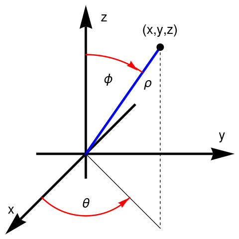
az = Graphics[{Black, Thickness[0.01], Arrowheads[0.1],
Arrow[{{0, -0.2}, {0, 1.2}}]}];
ax = Graphics[{Black, Thickness[0.01], Arrowheads[0.1], Arrow[{{0.4, 0}, {-0.65, -0.65}}]}]; ay = Graphics[{Black, Thickness[0.01], Arrowheads[0.1], Arrow[{{-0.4, 0}, {1.2, 0}}]}]; line = Graphics[{Blue, Thickness[0.01], Line[{{0, 0}, {0.6, 0.86}}]}]; line1 = Graphics[{Black, Dashed, Line[{{0.6, 0.86}, {0.6, -0.6}}]}]; line2 = Graphics[{Black, Line[{{0, 0}, {0.6, -0.6}}]}]; circle1 = Graphics[{Red, Thick, Circle[{0, 0}, 0.8, {Pi/2, 0.97}]}]; circle2 = Graphics[{Red, Thick, Circle[{0, 0}, 0.5, {-Pi/4, -3*Pi/4}]}]; ar1 = Graphics[{Red, Arrowheads[0.05], Arrow[{{0.36, 0.72}, {0.42, 0.67}}]}]; ar2 = Graphics[{Red, Arrowheads[0.05], Arrow[{{0.3, -0.395}, {0.35, -0.355}}]}]; disk = Graphics[Disk[{0.6, 0.86}, 0.03]]; tx = Graphics[{Black, Text[Style["x", 20], {-0.6, -0.45}]}]; ty = Graphics[{Black, Text[Style["y", 20], {1.1, 0.15}]}]; tz = Graphics[{Black, Text[Style["z", 20], {0.15, 1.1}]}]; tf = Graphics[{Black, Text[Style[\[Phi], 20], {0.18, 0.6}]}]; tt = Graphics[{Black, Text[Style[\[Theta], 20], {0, -0.4}]}]; tp = Graphics[{Black, Text[Style["(x,y,z)", 20], {0.6, 1.0}]}]; tr = Graphics[{Black, Text[Style[\[Rho], 20], {0.5, 0.57}]}]; Labeled[Show[ax, ay, az, line, line1, line2, circle1, circle2, ar1, ar2, disk, tx, ty, tz, tf, tt, tp, tr], "Spherical Coordinates"] |
|
| Spherical coordinates. | Mathematica code |
Unit vectors in spherical coordinates are
TableForm[Transpose[%]]
Dimension
Theorem 2 leads to the following definition.The basic field 𝔽 as a one-dimensional coordinate space. Here V = 𝔽; addition is addition in 𝔽 and multiplication by scalars is multiplication in 𝔽. The validity of the axioms of the linear space follows from the axioms of the field.
More generally, for any field 𝔽 and a subfield 𝔽 of it, 𝔽 can be interpreted as a linear space over 𝔽. For example, the field of complex numbers ℂ is a linear space over the field of real numbers ℝ, which in its turn is a linear space over the field of rational numbers ℚ.
The n-dimensional vector spaces constitute direct products 𝔽n = 𝔽 × 𝔽 × ċ × 𝔽. ■
To illustrate skew symmetric matrices, we present two examples: \[ \begin{bmatrix} \phantom{-}0&1&\phantom{-}2 \\ -1 & 0 &-3 \\ -2&3&\phantom{-}0 \end{bmatrix} \qquad \mbox{and} \qquad \begin{bmatrix} \phantom{-}0&\phantom{-}1&\phantom{-}2&3 \\ -1&\phantom{-}0&\phantom{-}4&5 \\ -2&-4 & \phantom{-}0 &6 \\ -3& -5& -6 & 0\end{bmatrix} . \] As we see from these two examples, there are n = 3 distinct skew symmetric 3×3 matrices and six skew symmetric 4×4 matrices. In general, there are n(n −1)/2 skew symmetric n × n matrices. Indeed, a skew symmetric matrix must have zero diagonal, All other entries are determined either by upper triangular entries or lower triangular entries because they differ by a sign. So we need to calculate the number of no zero entries above the main diagonal.
The first row contains n −1 terms, the second row contains n −2, and so on. Hence the total number of entries above the main diagonal is \[ m = \sum_{k=1}^{n-1} k = \frac{n\left( n-1 \right)}{2} . \] This is the dimension of the set of all n × n skew symmetric matrices.
Theorem 3: Let V be an n-dimensional vector space, and let S = { v1, v2, … , vn } be linearly independent set of vectors. Then S is a basis of V.
Each Pauli matrix is self-adjoint (Hermitian, so σj✶ = σj), and together with the identity matrix I (sometimes considered as the zeroth Pauli matrix σ₀), the Pauli matrices form a basis for the real vector space of 2 × 2 Hermitian matrices. This means that any 2 × 2 self-adjoint matrix can be written in a unique way as a linear combination of Pauli matrices, with all coefficients being real numbers. Hence, the vector space of self-adjoint 2 × 2 matrices over field of real numbers has dimension four. ■
Corollary 1: If a subset of a vector space V has fewer elements than the dimension of V, then this subset does not span V.
Corollary 2: If U is a subspace of the finite-dimensional vector space V, then U is also finite-dimensional and dim(U) ≤ dim(V) with equality if and only if U = V.
Theorem 4: Let V be an n-dimensional vector space, and let S = { v1, v2, … , vr }, r < n, be linearly independent set of vectors of V. Then there are vectors T = { vr+1, vr+2, … , vn } in V such that S ∪ T = { v1, v2, … , vn } is a basis of V.
To find the third linearly independent vector, we consider the matrix whose columns are a, b, and e₁ = i, e₂ = j, e₃ = k. So this matrix becomes \[ {\bf A} = \begin{bmatrix} 1 & -1 & 1 & 0 & 0 \\ 2 & 0 & 0 & 1 & 0 \\ 1 & 2 & 0 & 0 & 1 \end{bmatrix} . \] Using Gauss elimination, we transfer matrix A to its equivalent form \[ {\bf U} = \begin{bmatrix} \end{bmatrix} . \] ■
Theorem 5: Let V be a finite dimensional vector space over a field 𝔽 and U be a subspace of V. Then dimU ≤ dimV. Equality holds only when U = V.
When dimU = dimV. A basis of U is also a linearly independent subset of V. But dimV = n forces us to conclude that α is a basis of V also. Now we conclude that span(α) = U = V. This implies that U = V.
There is a subset of ℝn×n, known as the general linear group of degree n, that includes all n×n invertible matrices. This set is denoted as GL(n, ℝ) or GLₙ(𝔽) or just GLₙ when field is known. However, it is not a vector space with respect to addition of matrices because a sum of two matrices may be a singular matrix. For instance, \[ \begin{bmatrix} 1&0 \\ 0 &1 \end{bmatrix} + \begin{bmatrix} 0&1 \\ 1&0 \end{bmatrix} = \begin{bmatrix} 1&1 \\ 1&1 \end{bmatrix} . \] However, the general linear group is a vector space with respect to matrix multiplication, but we do not consider this operation over here. The set GL(n, ℝ) has the same basis β as ℝn×n; because every nonsingular square matrix is a linear combination of elementary matrices Ei,j. This allows us to claim that GL(n, ℝ) is of dimension n² while GLₙ ⊂ ℝn×n. Hence, a proper subset GL(n, ℝ) has the same dimension as the largest space ℝn×n.
The set of invertible matrices GLn(ℝ) is dense in the space of all square matrices ℝn×n because they have the same dimension, n². ■
A linear subspace V ⊂ ℝn×n of matrices with maximal rank r has dimension at most n r (see the article by H. Flanders). Nevertheless, the probability that a randomly generated matrix is singular---or nearly so, in the sense of having a condition number above a given threshold---is nonzero. When a matrix A is close to being singular, it is said to be ill-conditioned, and the associated problem A x = b is ill-posed. This underscores the importance of understanding numerical instability and condition numbers.
In case of 2 × 2 square matrices from ℝ2×2, the variety of singular matrices consists of matrices of the form \[ \begin{bmatrix} a & b \\ c & d \end{bmatrix} , \qquad a\,d = b\,c . \] So we have one condition, which eliminates one of the parameters. However, when we consider a vector subspace V involving singular matrices, one of these four parameters (𝑎, b, c, or d) can be chosen as 1 because a matrix can be multiplied by any nonzero number without changing its singularity (det = 0). Therefore, we have only at most two free parameters, and the dimension of the space of V is ≤ 2.
Let us be more specific and consider some examples. Say, we are given two singular matrices \( \displaystyle \quad {\bf A} = \begin{bmatrix} 1& 2 \\ 1& 2 \end{bmatrix} \quad \mbox{and} \quad {\bf B} = \begin{bmatrix} 2& 1 \\ 4& 2 \end{bmatrix} .\quad \) Their sum cannot belong to a vector space V ⊂ Sₙ because \[ \mathbf{A} + \mathbf{B} = \begin{bmatrix} 3& 3 \\ 5& 4 \end{bmatrix} \] is not a singular matrix. So vector space may contain only one of these two matrices. If V = span{A}, then din(V) = 1. A two-dimensional vector space containing singular matrices can be obtained by spanning a two-parameter matrix: \[ V = \mbox{span} \left\{ \begin{bmatrix} a& b \\ a& b \end{bmatrix} \right\} , \] where 𝑎 and b are some real numbers, not simulteneously equal to zero. ■
Corollary 1: Let V be a vector space over a field 𝔽 and W be a subspace of V. Let W⁰ = {φ ∈ V✶ : φ(v) = 0 for all v ∈ W} be the annihilator of subspace W. Then \[ \dim W + \dim W^0 ◦ = \dim V. \]
This is a linearly independent subset with n − m elements. Suppose that w✶ is an arbitrary element from W⁰. Since w✶ ∈ V⁰ and β✶ is a basis of V⁰, we find that w✶ = w✶(w₁) w₁✶ + w✶(w₂) w₂✶ + ⋯ + w✶(wn) wn✶. Since wj ∈ W for all 1 ≤ j ≤ m, we arrive at \( \displaystyle \quad {\bf w}^{\ast} = \sum_{i=m+1}^n {\bf w}^{\ast} \left( {\bf w}_i \right) {\bf w}_i^{\ast} . \quad \) This yields that { wm+1, … , wn } spans W⁰. Hence. dimW⁰ = n − m = n − dimW.
Complex Dimension
In mathematics, there are several varieties of dimensions to measure of the size of different objects. Although arbitrary fields are interesting and important in applications inside and outside of mathematics, we focus on two fields---real numbers (ℝ) and complex numbers (ℂ), partly because of their roles in physics and engineering. It is well known that real numbers are widely used in classical mechanics and geometry, complex numbers underlie the theories of electricity, magnetism, and quantum mechanics, all of which use linear algebra one way or another. Therefore, these two fields have a special place in linear algebra.
It should be noted that we use real and complex vector spaces only for theoretical analysis. In practice, we utilize only small part of these fields including rational numbers (ℚ) only because humans and computers do not operate with irrational numbers.
Recall that a complex number is a vector in ℝ² written in the form z = x + j y, with real components x, y ∈ ℝ. These real components are traditionally called real part and imaginary part of z, respectively. Notation x = Rez = ℜz and y = Imz = ℑz is widely used. The main reason of this form instead of standard form z = ix + j y is multiplication operation defined by \[ {\bf i}^2 = 1, \quad {\bf i}*{\bf j} = {\bf j}*{\bf i} = {\bf j} , \quad {\bf j}^2 = -1. \] Then we can drop i because it is just 1 for multiplication. Regular vector addition and multiplication just defined makes the field of complex numbers denoted by ℂ.
There is one more operation in the field of complex numbers---involution. There is no universal notation for complex conjugate---in mathematics it is denoted by overhead line, \( \displaystyle \overline{a + {\bf j}\,b} = a - {\bf j}\,b . \) In physics and engineering, the complex conjugate number is denoted by asterisk, \( \displaystyle (a + {\bf j}\,b)^{\ast} = a - {\bf j}\,b . \) In this tutorial, we mostly will follow the latter notation. For instance, \( \displaystyle (3 + 2\,{\bf j})^{\ast} = 3 - 2\,{\bf j} . \)
Theorem 7: If V is a complex vector space, then \[ \dim_{\mathbb{R}}V = 2\,\dim_{\mathbb{C}} V . \]
Suppose b1, b2, … , bn, bn+1, … , bn+m are elements in S and that \[ c_1 {\bf b}_1 + c_2 {\bf b}_2 + \cdots + c_n {\bf b}_n + {\bf j}\,c_{n+1} {\bf b}_{n+1} + \cdots + {\bf j}\,c_{n+m} {\bf b}_{n+m} = {\bf 0} , \] for real coefficients cj. Since coefficients cj and jcj are also complex, we can re-index the basis elements bi if necessary to rewrite the previous equation in the form \[ z_1 {\bf b}_1 + z_2 {\bf b}_2 + \cdots + z_k {\bf b}_k = {\bf 0} , \] where zi = ci + jcn+i and b1, b2, … , bkn are distinct elements of the nasis β. Since vectors from β are linearly independent, the coefficients in the equation above are all zeroes, zi = 0. This implies that all coefficients ci are also zeroes. This is enough to prove our claim.
A similar argument shows that any linear combination of elements from β over ℂ can be written as a linear combination of elements in β ∪ jβ over ℝ. This proves that β ∪ jβ is a basis for V over ℝ. The Theorem 5 follows.
Over the field of real numbers, the vector space \( \mathbb{C} \) of all complex numbers has dimension 2 because its basis consists of two elements \( \{ 1, {\bf j} \} . \)
In ℂ², we consider two vectors that generate a basis β = {(2, j), (j, −2)} ⊆ ℂ². To show their linearly independents, we consider \[ z_1 \left( 2, {\bf j} \right) + z_2 \left( {\bf j}, -2 \right) = \left( 0, 0 \right) = {\bf 0} , \] where z₁ and z₂ are some complex numbers. If this linear combination is equal to the zero vector, then its every component must be zero. We can solve the following system of equations over ℂ to find the coefficients \[ \begin{split} 2\,z_1 + z_2 {\bf j} &= 0, \\ z_1 {\bf j} - 2\,z_2 &= 0 . \end{split} \] Multiplying the first equation by j and second equation by −2 and adding the results, we obtain \[ 3\, z_2 = 0 \qquad \Longrightarrow \qquad z_2 = 0. \] Since it is a homogeneous equation, z₁ = 0. We check with Mathematica:
Now consider another basis jβ = {(2j, −1), (−1, −2j)}. Theorem 5 guarantees that β ∪ jβ is a basis for ℂ² as a vector space over ℝ. This means that we must be able to write arbitrary vector, for instance (3, 2), as a linear combination of elements in \[ \beta \cup {\bf j}\beta = \left\{ \left( 2, {\bf j} \right) , \left( {\bf j}, -2 \right) ,\left( 2{\bf j}, -1 \right) , \left( -1, -2{\bf j} \right) \right\} . \] Using real coefficients c>₁, c>₂, c>₃, c>₄, we get a relation \[ c_1 \left( 2, {\bf j} \right) + c_2 \left( {\bf j}, -2 \right) + c_3 \left( 2{\bf j}, -1 \right) + c_4 \left( -1, -2{\bf j} \right) = (3, 2) . \] We can find the coefficients by solving the following system of equations: \[ \begin{split} 2\, c_1 + c_2 {\bf j} + c_3 2{\bf j} - c_4 &= 3, \\ c_1 {\bf j} -2\,c_2 - c_3 -c_4 2{\bf j} &= 2 . \end{split} \] Separation of real and imaginary parts in both equations above yields \[ \begin{split} 2\, c_1 - c_4 &= 3, \\ c_2 + 2\,c_3 &= 0, \\ -2\,c_2 - c_3 &= 2, \\ c_1 -2\, c_4 &= 0. \end{split} \] Mathematica solves this system of equations in a blank of eye:
In order to show that {b1, b2, … , bn} is linearly dependent, we have to find k1, k2, … , kn ∈ 𝔽 not all zero such that \[ \sum_{j=1}^n k_j {\bf b}_j = {\bf 0} . \] This yields that \[ \sum_{j=1}^m k_j \left( \sum_{i=1}^m c_{i,j} {\bf v}_i \right) = {\bf 0} \qquad \iff \qquad \sum_{i=1}^m \left( \sum_{j=1}^n k_j c_{i,j} \right) {\bf v}_i = {\bf 0} . \] However, vectors {b1, b2, … , bn} form basis for V. The latter equation is valid when all coefficients are zeros. So \( \displaystyle \sum_{j=1}^n c_{i,j} k_J = 0 \) for each i such that 1 ≤ i ≤ m. This is a system of m homogeneous linear equations in n unknowns. Hence, there exists nontrivial solution say p1, p2, … , pn. This ensures that there exist scalars p1, p2, … , pn, not all zero such that \( \displaystyle \sum_{j=1}^n p_j {\bf b}_j = {\bf 0} \) and hence the set {b1, b2, … , bn} is linearly dependent.
Actually, we need to show the set β is linearly independent because β generates the set of all polynomials 𝔽[x]. Suppose opposite that there exists a finite subset S ⊂ β that is linearly dependent. Let xm be the highest power of x in S and let xn be the lowest power of x in S. Then there are scalars cn, … , cm not all zero, such that \[ c_n x^n + c_{n+1} x^{n+1} + \cdots + c_m x^m = 0 . \] Then the polynomial in the left-hand side is zero for all values of x. However, a polynomial of degree at most m cannot have more than m zeroes, but not identically. Therefore, this polynomial is identically zero and all coefficients are zeroes.
Another proof is more tedious. We can set x some values to be sure that the corresponding matrix is not singular (invertible). Then we get a homogeneous system of equations with invertible matrix that has only zero solution.
Let ℝE[x] and ℝO[x] be the sets of even and odd polynomials, respectively: \[ \mathbb{R}_{E}[x] = \left\{ p(x) \in \mathbb{R}[x]\, : \ p(-x) = p(x) \right\} \qquad \mbox{and} \qquad \mathbb{R}_{O}[x] = \left\{ p(x) \in \mathbb{R}[x]\, : \ p(-x) = -p(x) \right\} . \] We show that ℝE[x] is a subspace of ℝ[x] by checking the two closure properties:
- If p, q ∈ ℝE[x], then \[ \left( p + q \right) (-x) = p(-x) + q(-x) = p(x) + q(x) = \left( p + q \right) (x) . \] so p + q ∈ ℝE[x] too.
- If p ∈ ℝE[x] and λ ∈ ℝ, then \[ \left( \lambda\,p \right) (x) = \lambda\,p(x) = \lambda\left( p \right) (x) , \] so λp ∈ ℝE[x] too.
To find a basis of ℝE[x], we first notice that βE = { 1, x2, x4, … } ⊂ ℝE[x] because every element of βE is an even function. This set is also linearly independent since it is a subset of the linearly independent set β. To see that it spans ℝE[x], we notice that if \[ p(x) = a_0 + a_1 x + a_2 x^2 + a_3 x^3 + \cdots \in \mathbb{R}_E , \] then p(x) + p(−x) = 2 p(x), so \begin{align*} 2\,p(x) = p(x) + p(-x) \\ &= \left( a_0 + a_1 x + a_2 x^2 + a_3 x^3 + \cdots \right) + \left( a_0 - a_1 x + a_2 x^2 - a_3 x^3 + \cdots \right) \\ &= 2 \left( a_0 + a_2 x^2 + a_4 x^4 + \cdots \right) \in \mbox{span}\left( 1, x^2 , x^4 , \ldots \right) . \end{align*} It follows that p(x) = 𝑎₀ + 𝑎₂x2 + 𝑎₄x4 + ⋯ ∈ span(1, x2, x4, …), so the set { 1, x2, x4, … } spans ℝE[x], and is thus a basis of it.
A similar argument shows that ℝO[x] is a subspace of ℝ[x] with basis { x, x3, x5, … }.
You know from calculus that cosine function has an expansion \[ \cos x = 1 - \frac{x^2}{2} + \frac{x^4}{4!} - \frac{x^6}{6!} + \cdots = \sum_{n\ge 0} (-1)^n \frac{x^{2n}}{(2n)!} . \] Does it mean that cosine function belongs to ℝE[x] ? The answer is negative because the vector space ℝE[x] contains only linear combinations of finite terms. The cosine expansion contains infinite summation, but it is not defined in a vector space. ■
Infinite Dimensional Spaces
There is no restriction for using infinite dimensional spaces that are generated by infinite many linearly independent vectors. For example, the set V = ℭ(ℝ) of all continuous real-valued functions ℝ ↦ ℝ is a vector space. The zero function is the function that vanishes identicallyEach rational function has a representation f = p/q in simplified form where the polynomials p and q are relatively prime (have no common factor). In this form, q is uniquely determined up to a multiplication by a nonzero constant, and the finite set of its zeroes is known as the set of poles Pj of f. The value f(x) = p(x)/q(x) is well-defined provided x is not in this set Pf so that f defines a map \[ \mathbb{R} \setminus P_f \,\mapsto \,\mathbb{R} \] having for domain the complement of its set of poles. Since the real (or complex) field is infinite, the common domain of two rational functions is also infinite and with the usual definition for the sum and multiplication by scalars, the set of real (or complex) rational functions is a vector space. ■
We conclude this section with a proof that every vector space has a basis. Since it is based on Zorn's lemma, we need to review the associated terminology.
Let S be a set with a binary relation that we denote by "≤." If a pair {𝑎, b} belongs to S, we abbreviate it as 𝑎 ≤ b. A relation ≤ is an ordering on S provided it is
- transitive, meaning that if 𝑎, b, c in S satisfy 𝑎 ≤ b and b ≤ cb, then 𝑎 ≤ c; and
- antisymmetric, meaning that if 𝑎, b in S satisfy 𝑎 ≤ b and b ≤ 𝑎, then 𝑎 = b.
Zorn’s Lemma says that if every chain in a poset (S, ≤) has an upper bound in S, then S has a maximal element, that is, m in S such that if m ≤ 𝑎 for any 𝑎 in S, then 𝑎 = m. The poset in Example 14 has maximal element {𝑎, b, c}.
Let ₲ be a chain in S and let S₁ and S₂ be elements in ₲: S₁ and S₂ are linearly independent subsets of V, each containing S as a subset. As elements in a chain, either S₁ ⊆ S₂ or S₂ ⊆ S₁.
Let G be the union of the sets in ₲: G is a set of vectors, each of which belongs to a linearly independent set in a chain of linearly independent sets, each of which contains S as a subset.
We claim that G is linearly independent.
Suppose opposite that there are distinct v₁ , … , vk in G so that for some scalars c₁ , … , ck, we have \[ c_1 {\bf v}_1 + c_2 {\bf v}_2 + \cdots + c_k {\bf v}_k = {\bf 0} . \] As an element in G, each vi belongs to some Si in ₲. Since ₲ is a chain, we may assume that S₁ ⊆ S₂ ⊆ ⋯ ⊆ Sk. For i = 1, … , k, vi belongs to Sk. Since Sk is linearly independent, ci = 0 for i = 1, … , k. This is enough to establish that G is itself linearly independent, thus, that G belongs to ,I.S,/I., the collection of all linearly independent subsets of ,I.V,/I. containing S as a subset.
Since any element in ₲ is a subset of G, G is an upper bound for ₲. As every chain in S thus has an upper bound, Zorn’s Lemma guarantees the existence of a maximal element, β, in S. As a maximal linearly independent subset of V, β is a basis for V. Since S ⊆ β, the proof of the theorem is complete.
Since Theorem 9 holds in every vector space, we have established that every vector space has a basis.
Knowing that an infinite-dimensional vector space has a basis is often the best we can do. There are no algorithms for constructing bases in general.
- Let V be a finite dimensional vector space over a field 𝔽, and U₁, U₂, U₃ be any three subspaces of V. Then dim(U₁ + U₂ + U₃) ≤ dimU₁ + dimU₂ + dimU₃ − dim(U₁ ∩ U₂) − dim(U₂ ∩ U₃) − dim(U₁ ∩ U₃) + dim(U₁ ∩ U₂ ∩ U₃).
-
Let ℂ, ℝ, and ℚ denote the field of complex numbers, real numbers and rational
numbers, respectively. Show that
- ℂ is an infinite dimensional vector over ℚ.
- ℝ is an infinite dimensional vector over ℚ.
- The set {α + jβ, γ + jδ}, where j is the imaginary unit, j² = −1, is a basis of ℂ over ℝ if and only if αδ ≠ βγ. Hence, ℂ is a vector space of dimension 2 over ℝ.
- Show that the set of all polynomials ℝ[x] is a direct sum of polynomials of even degree ℝE[x] and odd degree ℝO[x].
- Let U = span{(1, 3, 2), (3, 2, -1), (1, 2, 1)} and W = span{(1, -3, 2), (2, -2, 4), (1, -2, 2)} be two subspaces of ℝ³. Determine the dimension and a basis for U + W, and U ∩ W. 7. Consider the following sum
- Let U = { (x₁, x₂, x₃, x₄) ∈ ℝ4 : x₂ + 2 x₃ + x₄ = 0 } and W = { (x₁, x₂, x₃, x₄) ∈ ℝ4 : x₁ + x₄ = 0, x₂ = 3 x₃} be subspaces of 4. Find bases and dimensions of UU, W, U ∩ W, and U + W.
- Let V = U + W for some finite dimensional subspaces U and W of V. If dimV = dinU + dimW, show that V = U ⊕ W.
- Let u ∈ ℝ be a transcendent number. Let U be the set of real numbers which are of the type c0 + c1u + ⋯ + ckuk, ci ∈ ℚ, k ≥ 0. Prove that U is an infinite dimensional subspace of ℝ over ℚ.
-
Assume that S = {v1, v2, … , vk} ⊆ V, where V is a vector space
of dimension n. Answer True/False to the following:
- If S is a basis of V then k = n.
- If S is linearly independent then k ≤ n.
- If S spans V, then k ≤ n.
- If S is linearly independent and k = n, then S spans V.
- If S spans V and k = n, then S is a basis for V.
- If A is a 5 by 5 matrix and det(A) = 1, then the first 4 columns of A span a 4 dimensional subspace of ℝ5.
-
Assume that V is a vector space of dimension n and S = {v1, v2, … , vk} ⊆ V. Answer True/False to the following:
- S is either a basis or contains redundant vectors.
- A linearly independent set contains no redundant vectors.
- If V = span{v1, v2, v3} and dim(V) = 2, then {v1, v2, v3} is a linearly dependent set.
- A set of vectors containing the zero vector is a linearly independent set.
- Every vector space is finite-dimensional.
- The set of vectors (j, 0), (0, j), (1, j) in ℂ² contains redundant vectors. Here j is the imaginary unit so j² = −1.
- Let p(x) = c₀ + c₁x + ⋯ + cm xm be a polynomial and A be an n×n matrix. Show that there exists a polynomial p(x) of degree at most n² for which p(A) = 0. Hint: use standard basis in the space ℝn×n. Compare your answer with the Cayley–Hamilton theorem.
- Show that a set of vectors {v1, v2, … , vn} in the vector space V is a basis if and only if it has no redundant vectors and dim(V) ≤ n.
- Anton, Howard (2005), Elementary Linear Algebra (Applications Version) (9th ed.), Wiley International
- Flanders, H., On Spaces of Linear Transformations with Bounded Rank, Journal of the London Mathematical Society, 1962, vol. 37, No. 1, pp. 10 -- 16.