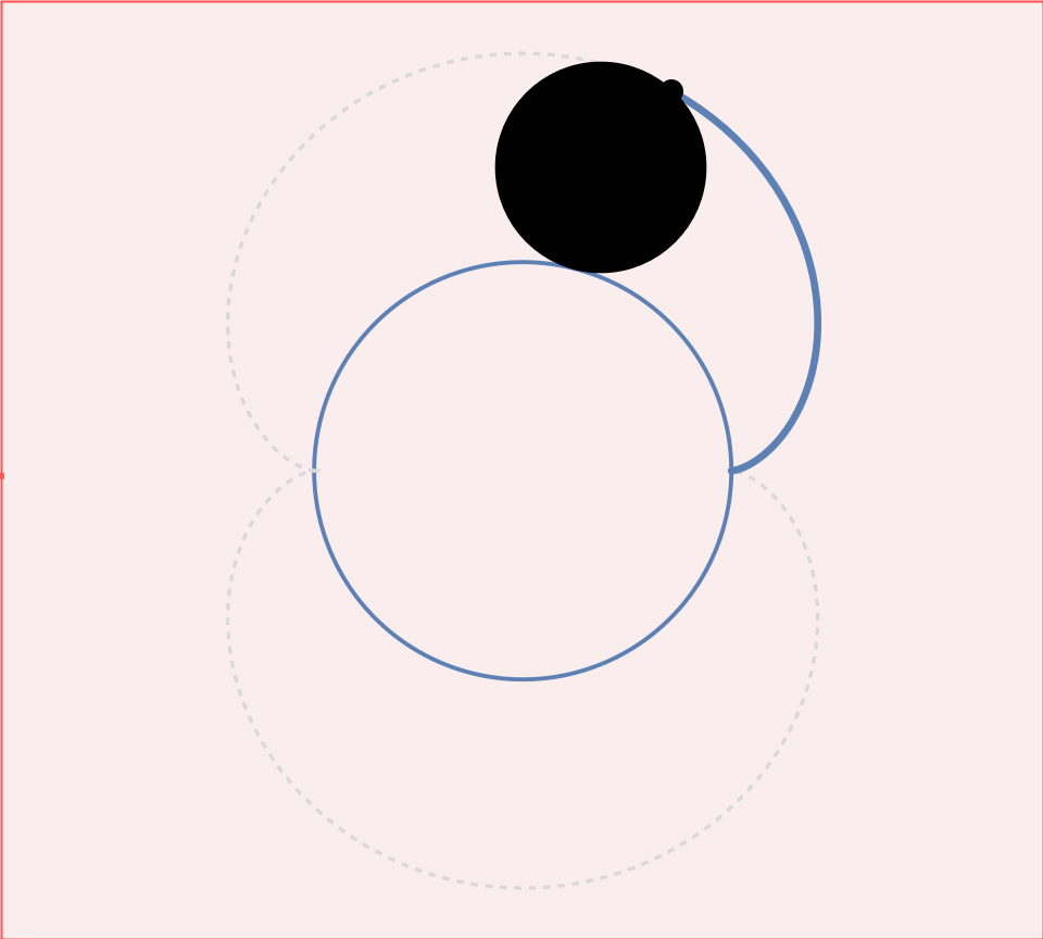
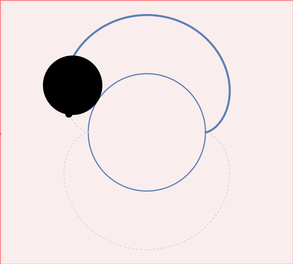
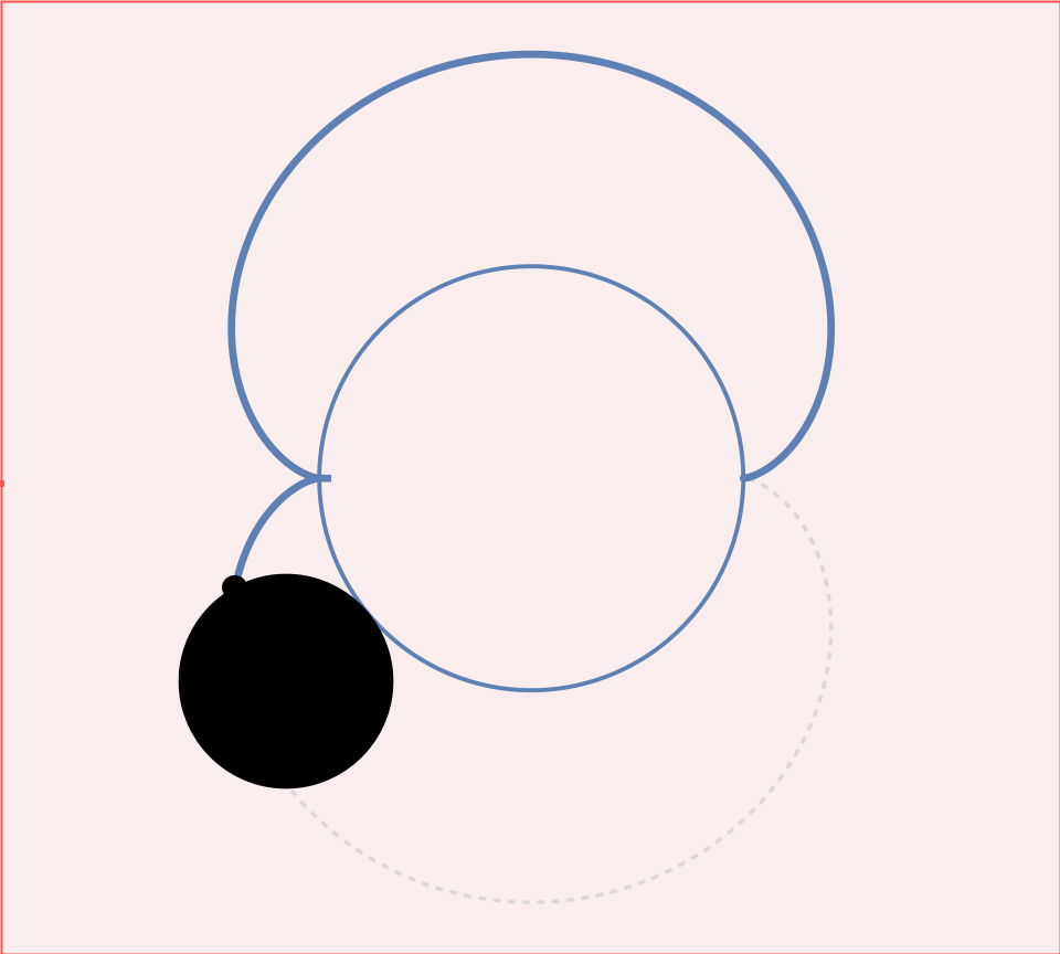
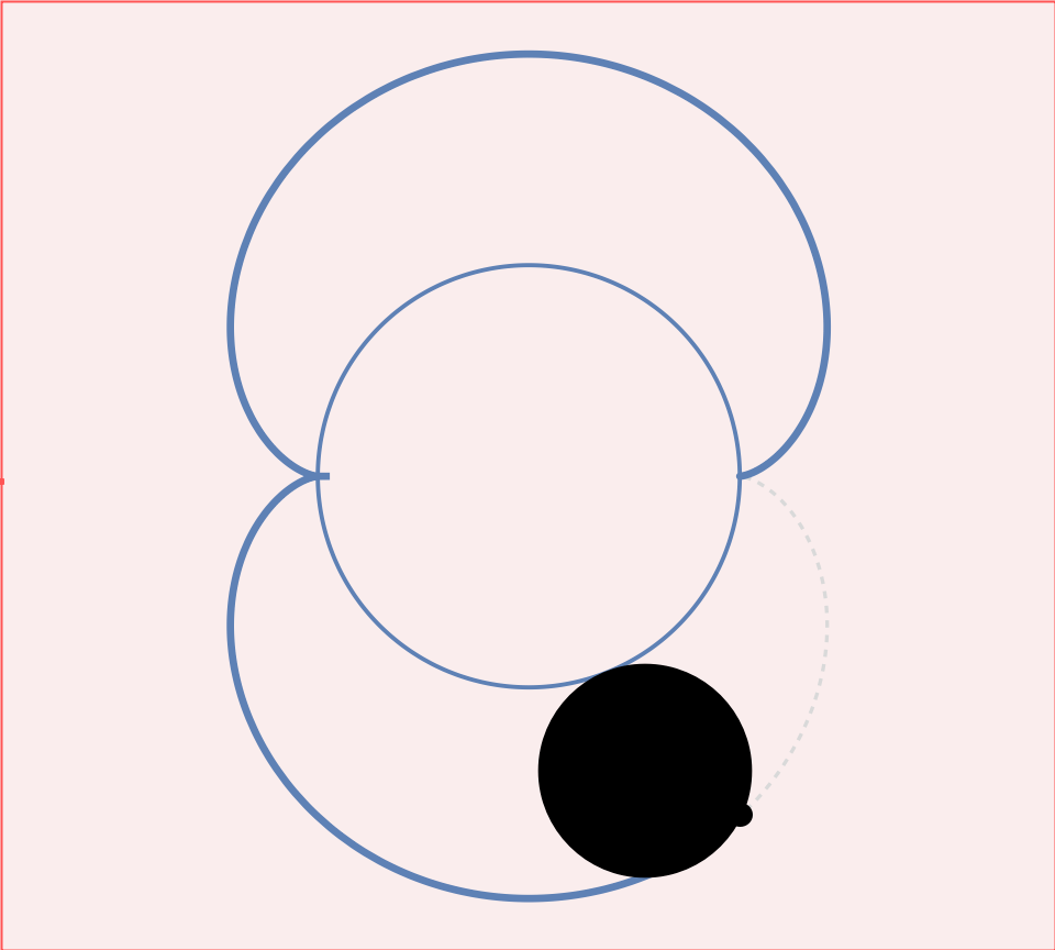
This section gives a combination of calculus, vectors, and parametric curves in an attempt to describe a
circle rolling along a parametric curve. The circles will have either a constant radius r or a variable radius. Our circles will be tangent
to the base curve along which they are rolling in both versions, since this will make the rolling
appear closest to the actual physical process. In order to visualize this process, a vector format
for our curves and their tangents is necessary.
Let a parametric curve in the plane be defined by
\[
x = f(t) \qquad\mbox{and}\qquad y = g(t) ,
\]
with t in the interval [𝑎, 𝑏].
Its vector format is x(t) = (f(t), g(t)). This is called the position vector field of the parametric curve. Its derivative vector field or tangent vector field is
Also, N(t) can be made length r, corresponding to the radius of our circles, by first making it a
unit vector field and then multiplying by r. Then the center vector field C(t) for our circles is
given by
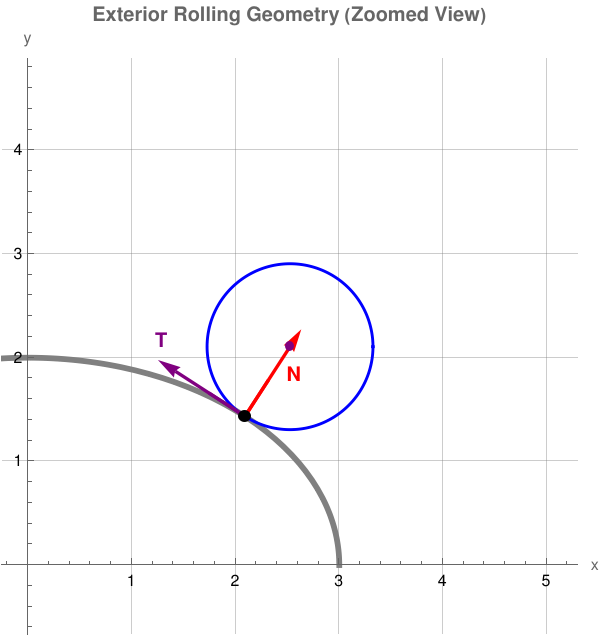
Here is an interactive Wolfram Mathematica script designed to give you an intuitive experience, this script uses Manipulate. It allows you to slide a parameter control t
along the interval [𝑎, 𝑏]
and watch the position vector x(t), the tangent vector T(t), the normal vector N(t), and your generated rolling circle tracking dynamically along the curve.
(* 1. Define your parametric ellipse functions f(t) and g(t) *)
f[t_] := 3 * Cos[t];
g[t_] := 2 * Sin[t];
(* Define full domain, though we will zoom in on a section *)
a = 0;
b = 2 * Pi;
(* 2. Define Vector Fields using the OUTWARD-pointing normal configuration *)
xVec[t_] := {f[t], g[t]};
TVec[t_] := {f'[t], g'[t]};
(* This variant flips the signs to point outwards from the ellipse interior *)
NVec[t_] := {g'[t], -f'[t]};
(* Center vector field C(t) for an outside rolling circle of radius r *)
CVec[t_, r_] := xVec[t] + (r / Norm[NVec[t]]) * NVec[t];
(* 3. Create the Interactive Visualization Environment *)
Manipulate[
Module[{
pos = xVec[tVal],
tangent = TVec[tVal],
normal = NVec[tVal],
center = CVec[tVal, rVal],
curvePlot, vectorsPlot, circlePlot
},
(* Plot a specific partial arc of the curve to emphasize the moving circle *)
curvePlot = ParametricPlot[{f[t], g[t]}, {t, Max[a, tVal - 1.5], Min[b, tVal + 1.5]},
PlotStyle -> Directive[Gray, Thickness[0.01]],
Axes -> True, AxesLabel -> {"x", "y"}, GridLines -> Automatic
];
(* Plot the rolling circle resting on the outside of the ellipse *)
circlePlot = ParametricPlot[
rVal * {Cos[s], Sin[s]} + center, {s, 0, 2 * Pi},
PlotStyle -> Directive[Blue, Thickness[0.005]]
];
(* Generate the vector arrows rooted strictly at the boundary coordinate *)
vectorsPlot = Graphics[{
(* Tangent Vector - Arrow (Green) *)
Text[Style["T", Purple, Bold, 12], pos + 0.6 * tangent/Norm[tangent] + {-0.3, 0.4}],
Purple, Thick, Arrow[{pos, pos + tangent/Norm[tangent]}],
(* Normal Vector pointing outwards toward the circle center - Arrow (Red) *)
Text[Style["N", Red, Bold, 12], pos + 0.6 * normal/Norm[normal] + {0.15, -0.1}],
Red, Thick, Arrow[{pos, pos + normal/Norm[normal]}],
(* Distinct Markers for Position and Center *)
Black, PointSize[0.02], Point[pos], (* Point x(t) on curve *)
Purple, PointSize[0.015], Point[center] (* Center C(t) of rolling circle *)
}];
(* Combine structures and clip the range tightly around the dynamic frame *)
Show[
curvePlot, circlePlot, vectorsPlot,
PlotRange -> {{center[[1]] - 2.5, center[[1]] + 2.5}, {center[[2]] - 2.5, center[[2]] + 2.5}},
AspectRatio -> Automatic,
ImageSize -> Medium,
PlotLabel -> Style["Exterior Rolling Geometry (Zoomed View)", 12, Bold]
]
],
(* Interactive Sliders for Student Control *)
{{tVal, 0.8, "Time Parameter (t)"}, a, b, Appearance -> "Labeled"},
{{rVal, 0.8, "Exterior Radius (r)"}, 0.3, 1.5, Appearance -> "Labeled"}
]
Figure 1.0: Illustration of formula (1).
If we now write C(t) = (h(t), k(t)), then our rolling circles are given by the parametric curve:
\begin{align*}
\left( x(s) , y(s) \right) &= \left( r\,\cos s + h(t) , r\,\sin s + k(t) \right)
\\
&= r \left( \cos (s) , \sin (s) \right) + \mathbf{C} (t) .
\end{align*}
As s varies in the interval [0, 2π], we move around this circle while we get one circle for each
fixed value t ∈ [𝑎, 𝑏]. In this situation, s is the variable that moves us around each circle while t
is the rolling variable that moves us from one circle to the next circle because it controls the location of the circles’ centers.
The formula for C(t) in \eqref{EqCircle.1} may appear complicated; however, if we take a minute to examine each piece, we should begin to see how simple it really is. Since C(t) is the center of the
circle that we wish to roll along the curve, we need to start on the curve, x(t) and move r units
perpendicular to x(t). Since N(t) is orthogonal to T(t), which in turn is tangent to x(t) we have
that N(t) is orthogonal to x(t). To proceed r units in the N(t) direction, we must first make N(t)
unit length by dividing it by its magnitude, then multiplying it by r. This gives the second piece of the sum found in Eq.\eqref{EqCircle.1}.
Example 1:
A cycloid is the geometric curve traced by a single point on the rim of a circle as it rolls along a straight line without slipping. Often called the "Helen of Geometers" due to the frequent historic quarrels it sparked among mathematicians, this shape possesses unique properties that solve legendary problems in physics and calculus.
Figure 1.1: Cycloid.
The base curve is simple in our case---it is just a horizontal line:
\[
x = t \qquad \mbox{and} \qquad y = 0 .
\]
Then the normal vector at every point x = t remains the same and it is collinear with the ordinate axis.
Let a circle of radius r
roll along the flat x-axis. We place the origin (0,0)
at the point where our tracing point P
initially touches the ground.
Let the circle rotate through an angle θ
(in radians). As the circle rolls:
The center of the circle C
moves horizontally. Because it rolls without slipping, the horizontal distance the center travels is exactly equal to the arc length rolled, which is
rθ.
The coordinates of the center C
at any angle θ
are (rθ, r).
Now, we find the position of the tracing point P(x, y)
relative to the moving center C. When the circle rotates clockwise by an angle θ:
The point P rotates backward relative to the center.
Measuring from the lowest point of the circle (the contact point), the vector from the center C
to the point P
points downward and backward.
With[{
angle = Pi/3,
radius = 1,
cx = 0,
cy = 1
},
(* Pre-calculate exact numeric coordinates to prevent errors *)
With[{
px = N[cx + radius * Sin[angle]],
py = N[cy - radius * Cos[angle]]
},
Graphics[{
(* Ground *)
GrayLevel[0.4],
Rectangle[{-2, -0.5}, {2, 0}],
(* Circle (Solid black border) *)
EdgeForm[{Thick, Black}], White,
Disk[{cx, cy}, radius],
(* Downward line from center: Isolated so only this line is dashed *)
{Dashed, Black, Line[{{cx, cy}, {cx, 0}}]},
(* Blue horizontal line: Fixed syntax with explicit thickness *)
Blue, AbsoluteThickness[4],
Line[{{px, py}, {cx, py}}],
(* Red point on the circle *)
Red, PointSize[Large],
Point[{px, py}],
(* Purple arrow (Resets thickness to look crisp) *)
Purple, AbsoluteThickness[2], Arrowheads[0.05],
Arrow[{{cx, cy}, {px, py}}],
(* Center Dot *)
Black, PointSize[Large],
Point[{cx, cy}],
(* Theta label *)
Text[Style["\[Theta]", 14, Italic, Black], {0.15, 0.65}],
(* Text label below the blue line *)
Text[Style["r sin(\[Theta])", 12, Italic, Blue], {px/2, py - 0.12}],
(* --- NEW EDITS --- *)
(* Label C for the Center of the Circle *)
Text[Style["C", 14, Bold, Black], {cx, cy + 0.2}],
(* Label P for the Reference Point *)
Text[Style["Q", 14, Bold, Black], {-0.2, py}],
Text[Style["P", 14, Bold, Red], {px + 0.27, py + 0}],
(* Counterclockwise Rotation Arrow placed near the top edge *)
(* Represents an arc from 50 degrees to 130 degrees at a radius of 1.25 *)
Darker[Green], AbsoluteThickness[2], Arrowheads[0.04],
Arrow[Table[
{cx + 1.25 * Cos[t], cy + 1.25 * Sin[t]},
{t, 50 Degree, 130 Degree, 5 Degree}
]]
},
Axes -> False,
PlotRange -> {{-3, 3}, {-1.5, 3}}
]
]
]
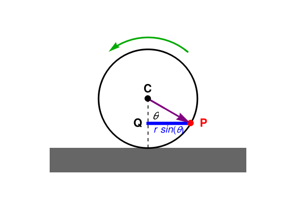
Figure 1.2: Horizontal displacement QP (in blue).
Using standard trigonometry from the center C:
The relative horizontal displacement is −r sinθ (see right triangle ▲CQP with angle ∡C = θ in Figure 1.2).
The relative vertical displacement CQ is −r cosθ.
Combining the absolute position of the center C
with the relative position of P:
\[
\begin{split}
x &= x_C + \Delta x = r\theta - r\,\sin\theta , \\
y &= y_C + \Delta y = r - r\,\cos\theta .
\end{split}
\]
Factoring out r
gives the standard parametric equations of a cycloid:
Cusps: The curve touches the flat baseline (y = 0) at periodic intervals where θ = 2πn, independently of the radius r.
Peaks: The maximum height of the curve is 2r, occurring at θ = π, 3π, ….
Applications: The cycloid solves both the brachistochrone problem (the path of fastest descent under gravity) and the tautochrone problem (where the time taken by an object sliding down the curve is independent of its starting point).
To find the distance the tracing point actually travels during one full rotation (0 to 2π), we use the parametric arc length formula:
The total length of one arch is exactly 8
times the radius of the rolling circle.
(* 1. Setup Parameters & Styled Functions *)
R = 1;
cycloidX[t_] := R*(t - Sin[t]);
cycloidY[t_] := R*(1 - Cos[t]);
(* Colors *)
cycloidColor = RGBColor["#FF5722"]; (* Vibrant Orange-Red *)
circleColor = RGBColor["#009688"]; (* Deep Teal *)
accentColor = RGBColor["#3F51B5"]; (* Indigo point *)
(* 2. Generate Frames with Sleek Aesthetic Elements *)
frames = Table[
Show[
(* Background Grid and Full Path Skeleton *)
ParametricPlot[{cycloidX[t], cycloidY[t]}, {t, 0, 2 Pi},
PlotStyle -> Directive[GrayLevel[0.85], Dashed],
PlotRange -> {{-0.5, 2 Pi + 0.5}, {-0.1, 2.2}},
Axes -> True,
Ticks -> {{0, {Pi, "\[Pi]"}, {2 Pi, "2\[Pi]"}}, {0, 1, 2}},
AspectRatio -> Automatic,
Background -> GrayLevel[0.98],
ImageSize -> Large
],
(* Active Growing Cycloid Segment *)
ParametricPlot[{cycloidX[t], cycloidY[t]}, {t, 0, Max[0.001, maxT]},
PlotStyle -> Directive[cycloidColor, Thickness[0.007], CapForm["Round"]]
],
(* Rolling Circle Assembly *)
Graphics[{
(* Moving Base / Floor Line *)
Directive[Black, Thickness[0.002]],
Line[{{-1, 0}, {2 Pi + 1, 0}}],
(* Rolling Circle Outline and Center Shading *)
Directive[circleColor, Thickness[0.004]],
Circle[{R*maxT, R}, R],
Directive[Opacity[0.1], circleColor],
Disk[{R*maxT, R}, R],
(* Vertical reference line showing current ground contact *)
Directive[GrayLevel[0.5], Dotted, Thickness[0.002]],
Line[{{R*maxT, 0}, {R*maxT, R}}],
(* Rotating Spoke/Radius Line *)
Directive[circleColor, Thickness[0.003]],
Line[{{R*maxT, R}, {cycloidX[maxT], cycloidY[maxT]}}],
(* Center Point *)
circleColor, PointSize[0.015], Point[{R*maxT, R}],
(* The Tracing Point *)
accentColor, PointSize[0.022], Point[{cycloidX[maxT], cycloidY[maxT]}]
}]
],
{maxT, 0, 2 Pi, 2 Pi/80} (* Increased frames to 80 for smoother motion *)
];
(* 3. Export to High-Quality Loop GIF *)
Export["custom_cycloid_animation.gif", frames,
"AnimationRepetitions" -> Infinity,
"DisplayDurations" -> 0.04
]
How to use this code:
Copy and paste the script directly into a blank Mathematica notebook.
Select the cell and press Shift + Enter to run it.
Mathematica will generate the frames locally and save a high-quality file named cycloid_animation.gif directly inside your current working directory (you can find or change this path using the command Directory
■
End of Example 1
Example 2:
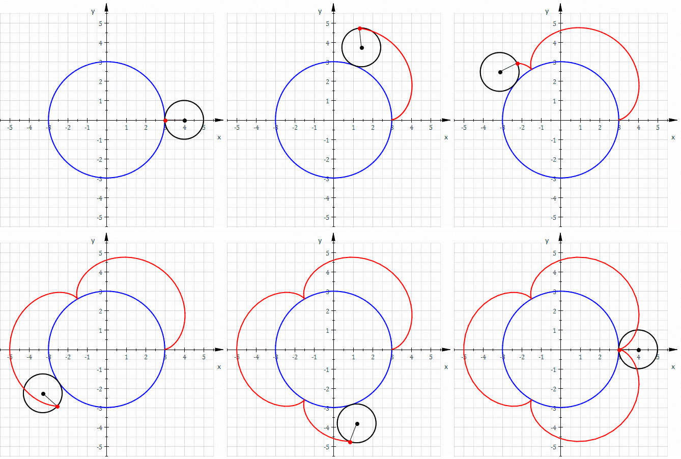
An epicycloid is a plane curve made by tracking the path of a chosen point on the edge of a circle as it rolls around the outside of another fixed circle without slipping.
Figure 2.1: Epicycloid.
Let a stationary base circle have a radius of R centered at the origin (0,0). A smaller rolling circle with a radius of r rolls along its outer circumference without slipping.
We trace a point P starting on the outer rim where the two circles touch on the positive x-axis. As the rolling circle moves through an angle θ around the center of the base circle:
The center C(xc, yc) of the moving circle is located at a distance of R + r from the origin. Its coordinates are:
\[
x_c = \left( R + r \right) \cos\theta , \qquad y_c = \left( R + r \right) \sin\theta .
\]
Because it rolls without slipping, the arc length traveled on both circles must be equal (Rθ = rα, where α is the internal rotation angle of the rolling circle). The position of P(x, y) relative to the center C(xc, yc) depends on the total accumulated angle of rotation of the rolling radius, which is
To understand how the latter formula connecting ϕ and θ is derived, we need to look closely at the condition for rolling without slipping and track the angles from two different points of view: an observer standing outside the system (the fixed base frame) and the moving center C of the rolling circle.
Let’s set up the system with a large stationary base circle of radius R
centered at the origin, and a smaller circle of radius r
rolling along its outside edge.
θ: The angle of the center of the rolling circle relative to the origin. This is how far the small circle has traveled around the large circle.
The point of contact on the large circle has traveled an arc length of:
\[
s_{\mbox{base}} = R\,\theta .
\]
Because the small circle rolls without slipping, the length of the arc it has rolled out along its own circumference must be exactly equal to the distance it covered on the large base circle.
If we let α
be the angle that the small circle has rotated relative to the moving line connecting the two centers, its internal arc length is: srolling = rα.
The angle α
only measures how much the circle has spun relative to the line connecting the centers. However, that center line itself is also rotating around the origin at an angle of θ.
To find the total, absolute rotation angle ϕ
of the tracking point relative to the fixed horizontal x-axis (the base frame), we have to add these two rotations together:
Combining the moving center coordinates with the trigonometric rotation adjustments gives the parametric equations for an epicycloid:
\[
\begin{split}
x (\theta ) &= \left( R + r \right) \cos\theta - r\,\cos \left( \frac{R+r}{r}\,\theta \right) ,
\\
y (\theta ) &= \left( R + r \right) \sin\theta - r\,\sin \left( \frac{R+r}{r}\,\theta \right) .
\end{split}
\]
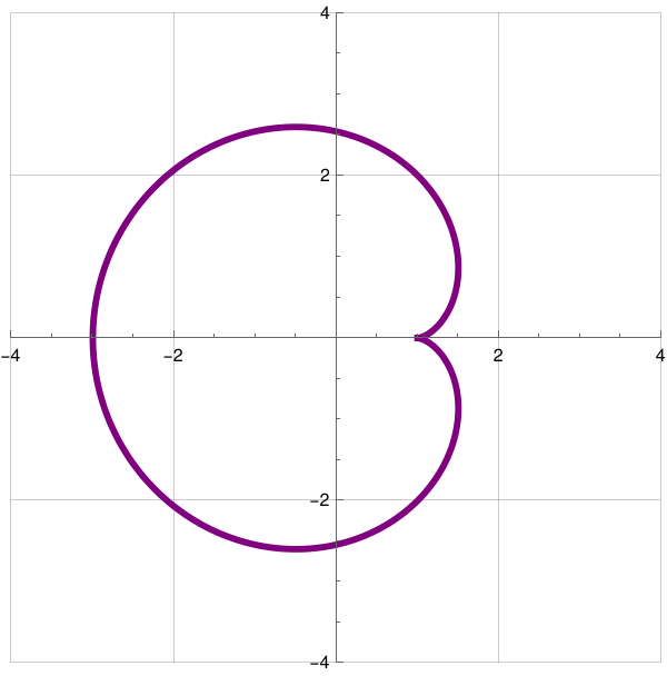
The following Mathematica code creates a cardioid (a heart-shaped epicycloid) by setting R = 2 and r = 1 (a 2:1 ratio). You can easily change these parameters at the top of the script to create different shapes (e.g., setting R = 2, r = 0.5 creates a nephroid).
(* 1. Define Radii Parameters (R = base circle, r = rolling circle) *)
R = 2;
r = 1;
(* Custom Epicycloid Equations *)
epicycloidX[t_] := (R + r)*Cos[t] - r*Cos[((R + r)/r)*t];
epicycloidY[t_] := (R + r)*Sin[t] - r*Sin[((R + r)/r)*t];k
(* 2. Build the Frame List *)
frames = Table[
Show[
(* Static Background Base Circle & Full Path Outline *)
ParametricPlot[{R*Cos[t], R*Sin[t]}, {t, 0, 2 Pi},
PlotStyle -> Directive[baseCircleColor, Thickness[0.004]],
PlotRange -> {-(R + 2 r) - 0.5, (R + 2 r) + 0.5},
Axes -> False,
AspectRatio -> Automatic,
Background -> GrayLevel[0.98],
ImageSize -> Large
],
(* Overlay a faint ghost line of the total expected epicycloid *)
ParametricPlot[{epicycloidX[t], epicycloidY[t]}, {t, 0, 2 Pi},
PlotStyle -> Directive[GrayLevel[0.85], Dashed]
],
(* Active Growing Epicycloid Curve *)
ParametricPlot[{epicycloidX[t], epicycloidY[t]}, {t, 0, Max[0.001, maxT]},
PlotStyle -> Directive[traceColor, Thickness[0.007], CapForm["Round"]]
],
(* Dynamic Visual Components *)
Graphics[{
(* Moving Center of Rolling Circle *)
With[{cX = (R + r)*Cos[maxT], cY = (R + r)*Sin[maxT]}, {
(* The rolling circle body *)
Directive[rollingColor, Thickness[0.004]],
Circle[{cX, cY}, r],
Directive[Opacity[0.08], rollingColor],
Disk[{cX, cY}, r],
(* Radial spoke line connecting roller center to trace point *)
Directive[rollingColor, Thickness[0.003]],
Line[{{cX, cY}, {epicycloidX[maxT], epicycloidY[maxT]}}],
(* Roller center coordinate point *)
rollingColor, PointSize[0.015], Point[{cX, cY}]
}],
(* The main active tracing point on the rim *)
traceColor, PointSize[0.022], Point[{epicycloidX[maxT], epicycloidY[maxT]}]
}]
],
{maxT, 0, 2 Pi, 2 Pi/100}
];
(* 3. Export to Seamless Loop GIF *)
Export["epicycloid_animation.gif", frames,
"AnimationRepetitions" -> Infinity,
"DisplayDurations" -> 0.04
]
To clarify the geometry first: an epicycloid with R = r
creates a cardioid (1 cusp), while an epicycloid with R = 2r
creates a nephroid (2 cusps).
Below are two options for Wolfram Mathematica code. The first plots both curves statically side-by-side, and the second creates an interactive animation showing the transition from the cardioid to the R = 2r
curve.
Paste it directly into a clean cell in a Mathematica Notebook.
Press Shift + Enter to evaluate and generate the graphics.
Figure 2.6: Cardioid (R = r).
■
End of Example 2
Example 3:
An ellipse centered at the origin (0,0)
with a horizontal semi-major axis 𝑎
and a vertical semi-minor axis b
is defined parametrically by the following two equations:
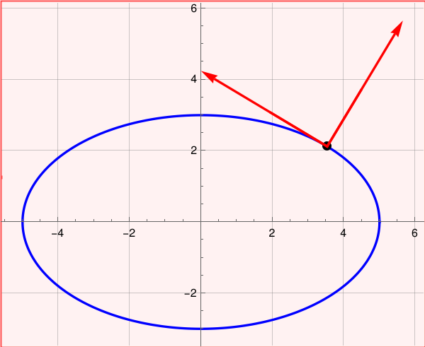
We plot the tangent vector and the normal vector at a particular point t₀ of the ellipse:
(* 1. Define the parameters *)
a = 5; (* Horizontal radius *)
b = 3; (* Vertical radius *)
t0 = Pi/4; (* Chosen parameter point *)
(* 2. Define the position, tangent, and normal vectors *)
R[t_] := {a*Cos[t], b*Sin[t]};
T[t_] := {-a*Sin[t], b*Cos[t]};
Nvec[t_] := {b*Cos[t], a*Sin[t]}; (* Outward normal vector *)
(* 3. Calculate exact coordinates at t0 *)
basePoint = R[t0];
tangentDir = T[t0];
normalDir = Nvec[t0];
(* 4. Create the plots and combine them *)
ellipsePlot = ParametricPlot[R[t], {t, 0, 2 Pi},
PlotStyle -> Directive[Blue, Thick],
AspectRatio -> Automatic,
GridLines -> Automatic];
vectorsPlot = Graphics[{
(* The point of intersection *)
Black, PointSize[Large], Point[basePoint],
(* Tangent Vector (Red) *)
Red, Thick, Arrow[{basePoint, basePoint + tangentDir}],
(* Normal Vector (Dark Green) *)
DarkGreen, Thick, Arrow[{basePoint, basePoint + normalDir}]
}];
(* Display them together *)
Show[ellipsePlot, vectorsPlot, PlotRange -> All]
ellipse =
ParametricPlot[{5 Cos[t], 3 Sin[t]}, {t, 0, 2 Pi},
PlotStyle -> {Black, Thickness[0.01]}]
Ellipse and tangent and normal vectors.
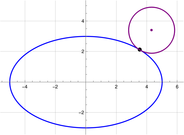
Mathematically, the center of the circle C that touches the ellipse externally is calculated as
\[
C = \mathbf{x}\left( t_0 \right) + r \cdot \hat{\bf n}\left( t_0 \right) ,
\]
where x(t₀) is the point on the ellipse, r
is the chosen radius of the circle, and n
is the normalized (unit) outward normal vector.
(* 1. Define the parameters *)
a = 5; (* Horizontal radius of ellipse *)
b = 3; (* Vertical radius of ellipse *)
t0 = Pi/4; (* Point of tangency *)
r = 1.5; (* Radius of the external circle *)
(* 2. Define position vector and outward unit normal vector *)
R[t_] := {a*Cos[t], b*Sin[t]};
Nvec[t_] := {b*Cos[t], a*Sin[t]};
unitN[t_] := Nvec[t] / Norm[Nvec[t]];
(* 3. Compute the tangency point and the circle's center *)
basePoint = R[t0];
circleCenter = basePoint + r * unitN[t0];
(* 4. Generate and combine the plots *)
ellipsePlot = ParametricPlot[R[t], {t, 0, 2 Pi},
PlotStyle -> Directive[Blue, Thick],
AspectRatio -> Automatic,
GridLines -> Automatic];
circlePlot = Graphics[{
(* Tangency point *)
Black, PointSize[Large], Point[basePoint],
(* Center of the touching circle *)
Purple, PointSize[Medium], Point[circleCenter],
(* The external circle *)
Purple, Thick, Circle[circleCenter, r]
}];
Show[ellipsePlot, circlePlot, PlotRange -> All]
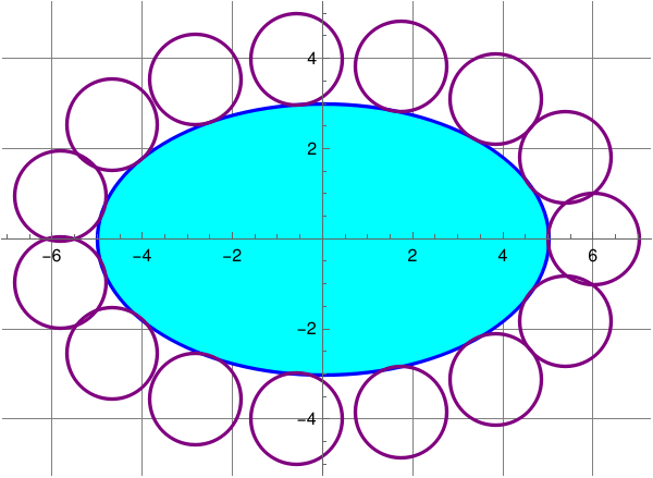
Figure 3.2: A circle touching Ellipse.
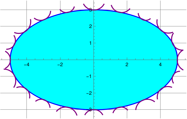
Now we plot the same ellipse together with some pieces of circles that touches the ellipse outside.
(* 1. Define the core ellipse parameters *)
a = 5; (* Horizontal radius *)
b = 3; (* Vertical radius *)
(* 2. Generate the list of 20 points and 20 example radii *)
tVals = Table[k * Pi / 10, {k, 1, 20}];
radiiVals = Table[0.4 + 0.3 * Abs[Sin[k]], {k, 1, 20}];
(* 3. Define position vector and outward unit normal vector functions *)
R[t_] := {a*Cos[t], b*Sin[t]};
Nvec[t_] := {b*Cos[t], a*Sin[t]};
unitN[t_] := Nvec[t] / Norm[Nvec[t]];
(* 4. Single-block graphics rendering pipeline *)
Graphics[{
(* A. Fill the interior of the ellipse with LightCyan *)
LightCyan, Disk[{0, 0}, {a, b}],
(* B. Draw the sharp, bold blue perimeter line *)
Blue, Thick, Circle[{0, 0}, {a, b}],
(* C. Generate and style the 20 touching purple arcs *)
Purple, Thick,
Table[
Module[{t = tVals[[k]], rOuter = radiiVals[[k]], basePoint, circleCenter, baseAngle, dirVect},
basePoint = R[t];
dirVect = unitN[t];
circleCenter = basePoint + rOuter * dirVect;
(* Calculate the baseline vector heading *)
baseAngle = ArcTan @@ (-dirVect);
(* Render the arc using Circle[{center}, radius, {startAngle, endAngle}] *)
Circle[circleCenter, rOuter, {baseAngle - Pi/3, baseAngle + Pi/3}]
],
{k, 1, 20}]
},
(* Global canvas settings *)
Axes -> True,
GridLines -> Automatic,
AspectRatio -> Automatic,
PlotRange -> All
]
Figure 3.3: Pieces of circles touching Ellipse.
Now we plot circles of fixed radius touching the ellipse outside:
(* 1. Define the core ellipse dimensions *)
a = 5; (* Horizontal radius *)
b = 3; (* Vertical radius *)
(* 2. Generate the list of 15 points and set a FIXED radius for all circles *)
nCircles = 15;
tVals = Table[k * 2 * Pi / nCircles, {k, 1, nCircles}];
fixedRadius = 1.3; (* Change this single number to resize all circles *)
(* 3. Define position vector and outward unit normal vector functions *)
R[t_] := {a*Cos[t], b*Sin[t]};
Nvec[t_] := {b*Cos[t], a*Sin[t]};
unitN[t_] := Nvec[t] / Norm[Nvec[t]];
(* 4. Single-block graphics rendering pipeline *)
Graphics[{
(* A. Fill the interior of the ellipse with solid Cyan *)
Cyan, Disk[{0, 0}, {a, b}],
(* B. Draw the sharp, bold blue perimeter line *)
Blue, Thick, Circle[{0, 0}, {a, b}],
(* C. Generate and style the 15 touching FULL purple circles *)
Purple, Thick,
Table[
Module[{t = tVals[[k]], basePoint, circleCenter, dirVect},
basePoint = R[t];
dirVect = unitN[t];
circleCenter = basePoint + fixedRadius * dirVect;
(* Render the full circle (baseAngle calculation is no longer needed) *)
Circle[circleCenter, fixedRadius]
],
{k, 1, nCircles}]
},
(* Global canvas settings *)
Axes -> True,
GridLines -> Automatic,
AspectRatio -> Automatic,
PlotRange -> All
]
is the incomplete Elliptic integral of the second kind with parameter k. In Mathematica, it can be evaluated as
arcLength[t_, a_, b_] := b * EllipticE[t, 1 - a^2/b^2]
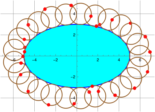
Now we roll a unit circle (of radius 1) counterclockwise along the ellipse with making point on its circumferance. To accurately model a circle rolling without slipping along the ellipse perimeter, the rotation angle must be proportional to the actual distance traveled along the curve—which is the arc length governed by the incomplete elliptic integral of the second kind.
* 1. Define core ellipse and circle properties *)
a = 5; (* Horizontal radius *)
b = 3; (* Vertical radius *)
r = 1.0; (* Fixed radius of brown circles *)
nCircles = 25; (* Total number of circles *)
(* 2. Generate the parameter values for the 25 positions *)
tVals = Table[k * 2 * Pi / nCircles, {k, 1, nCircles}];
(* 3. Define position vector and outward unit normal vector functions *)
R[t_] := {a*Cos[t], b*Sin[t]};
Nvec[t_] := {b*Cos[t], a*Sin[t]};
unitN[t_] := Nvec[t] / Norm[Nvec[t]];
(* 4. Define the exact arc length function using the Elliptic Integral *)
s[t_] := b * EllipticE[t, 1 - a^2/b^2];
(* 5. Single-block graphics rendering pipeline *)
Graphics[{
(* A. Fill the interior of the ellipse with solid Cyan *)
Cyan, Disk[{0, 0}, {a, b}],
(* B. Draw the bold blue ellipse boundary line *)
Blue, Thick, Circle[{0, 0}, {a, b}],
(* C. Generate the 25 brown circles and their rolling red marker disks *)
Table[
Module[{t = tVals[[k]], basePoint, circleCenter, rollingAngle, redPoint},
(* Compute the touching point on the ellipse *)
basePoint = R[t];
(* Compute the center of the brown circle *)
circleCenter = basePoint + r * unitN[t];
(* The true inclination angle from the initial position is arc length / radius *)
rollingAngle = s[t] / r;
(* Position the red disk on the circumference based on the true rolling angle *)
redPoint = circleCenter + r * {Cos[rollingAngle], Sin[rollingAngle]};
{
(* Draw the brown circle *)
Brown, Thick, Circle[circleCenter, r],
(* Draw the red marker disk (radius 0.15) *)
Red, Disk[redPoint, 0.15]
}
],
{k, 1, nCircles}]
},
(* Global canvas settings *)
Axes -> True,
GridLines -> Automatic,
AspectRatio -> Automatic,
PlotRange -> All
]
Figure 3.5: A circle rolling Ellipse.
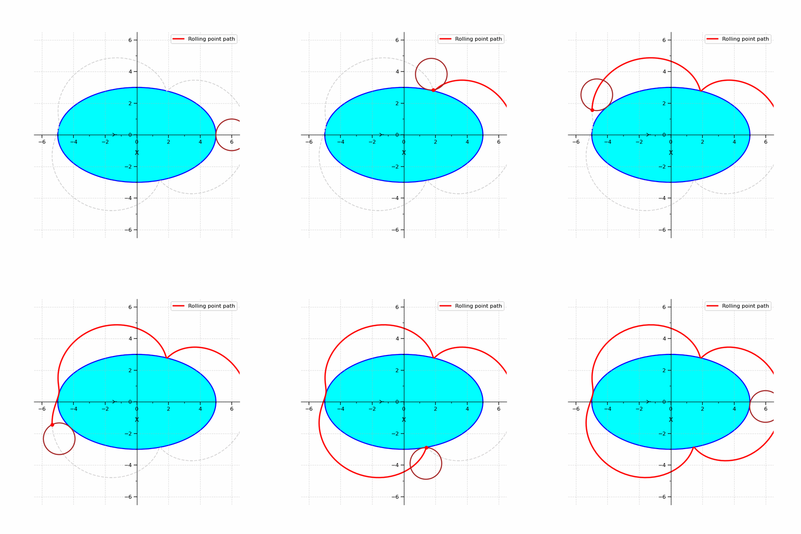
We want to add a trace line to the plot that shows the continuous path the red dot/point carves out as it rolls all the way around.
While a unit circle rolls around the ellipse, the red dots will trace a physically accurate cycloid-like progression that reflects the true geometry of the ellipse.
(* 1. Define core ellipse and circle properties *)
a = 5; (* Horizontal radius *)
b = 3; (* Vertical radius *)
r = 1.0; (* Fixed radius of brown circles *)
nCircles = 35; (* Total number of discrete brown circles to show *)
(* 2. Define geometry and rolling physics functions *)
R[t_] := {a*Cos[t], b*Sin[t]};
Nvec[t_] := {b*Cos[t], a*Sin[t]};
unitN[t_] := Nvec[t] / Norm[Nvec[t]];
s[t_] := b * EllipticE[t, 1 - a^2/b^2];
(* 3. Define the exact path vector of the rolling red marker point *)
redPath[t_] := Module[{circleCenter, rollingAngle},
circleCenter = R[t] + r * unitN[t];
rollingAngle = s[t] / r;
circleCenter + r * {Cos[rollingAngle], Sin[rollingAngle]}
];
(* 4. Pre-calculate 500 dense points to draw the continuous red curve *)
denseTrajectory = Table[redPath[t], {t, 0, 2 * Pi, 2 * Pi / 500}];
(* 5. Discrete positions for the 35 brown circles *)
tVals = Table[k * 2. * Pi / nCircles, {k, 1, nCircles}];
(* 6. Single-block graphics rendering pipeline *)
Graphics[{
(* A. Fill the interior of the ellipse with solid Cyan *)
Cyan, Disk[{0, 0}, {a, b}],
(* B. Draw the bold blue ellipse boundary line *)
Blue, Thick, Circle[{0, 0}, {a, b}],
(* C. Draw the continuous smooth red trajectory curve *)
Red, AbsoluteThickness[2.5], Line[denseTrajectory],
(* D. Generate the 35 brown circles and their corresponding red dots *)
Table[
Module[{t = tVals[[k]], basePoint, circleCenter, redPoint},
basePoint = R[t];
circleCenter = basePoint + r * unitN[t];
redPoint = redPath[t];
{
(* Draw the brown circle *)
Brown, Thickness[Small], Circle[circleCenter, r],
(* Draw the red marker disk on top *)
Red, Disk[redPoint, 0.12]
}
],
{k, 1, nCircles}]
},
(* Global canvas settings *)
Axes -> True,
GridLines -> Automatic,
AspectRatio -> Automatic,
PlotRange -> All
]
Figure 3.6: A cycloid-like curve formed by rolling circle.
■
End of Example 3
Example 4:
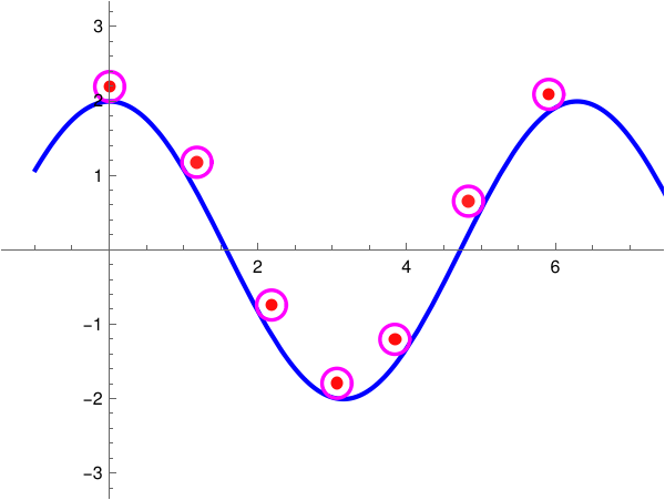
We choose the base parametric curve as y = 2 cos(x). This curve can be paratmetrized as
\[
x = t, \qquad y = 2\,\cos (t) , \qquad t \in [0, 2\pi ] ,
\]
Next, we use the Manipulate command to create an animation of these circles “rolling” along the cosine curven. The arc length s(t) from τ = 0 to τ = t is given by the integral
The elliptic integral of the second kind is implemented in the Wolfram Language as EllipticE[phi, m] (note the use of the parameter m = k² instead of the modulus k).
Manipulate[
Module[{basePoint, normalVect, circleCenter, currentArc, rollAngle, redPoint},
(* 1. Position on the cosine curve *)
basePoint = {tval, 2 * Cos[tval]};
(* 2. Upward unit normal vector to the cosine curve *)
normalVect = {2 * Sin[tval], 1} / Sqrt[1 + 4 * Sin[tval]^2];
(* 3. Exact center of the rolling circle *)
circleCenter = basePoint + r * normalVect;
(* 4. True arc length of y = 2*Cos[t] from 0 to tval *)
currentArc = EllipticE[tval, -4];
(* 5. Clockwise rotation angle based on distance traveled *)
rollAngle = -currentArc / r;
(* 6. Position of the red marker point on the circle's edge *)
redPoint = circleCenter + r * {Cos[rollAngle], Sin[rollAngle]};
Graphics[{
(* A. Draw the baseline Cosine Curve *)
Thick, Blue, Line[Table[{x, 2 * Cos[x]}, {x, -1, 7, 0.05}]],
(* B. Draw the rolling circle *)
Brown, Thick, Circle[circleCenter, r],
(* C. Draw a radius line to visually show the circle spinning *)
Darker[Gray], Line[{circleCenter, redPoint}],
(* D. Mark the center point with a red '+' *)
Red, Thick, Text["+", circleCenter],
(* E. Draw the red marker point on the circumference *)
Red, Disk[redPoint, 0.05]
},
Axes -> True,
GridLines -> Automatic,
PlotRange -> {{-1, 7}, {-3, 3.5}},
AspectRatio -> Automatic
]
],
(* Control Slider Settings *)
{{tval, 0, "Location (t)"}, 0, 2 * Pi, Pi / 64},
(* Define the radius globally upon initialization *)
Initialization :> (r = 0.2;)
]
■
End of Example 4
Example 5:
We modify the calculations given in the previous example with a nonconstant radius. In particular, we are
going to choose the radius to be 1/κ, where κ is the curvature of the function.
Curvature is denoted by the Greek letter kappa and is defined as the magnitude of the rate of change of the unit tangent vector with respect to arc length.
Curvature is inversely proportional to the radius of the "osculating circle" (the circle that best hugs the curve at that specific point).
For a regular planar curve given by y = f(x), the curvature
κ at any point x
is calculated using its first and second derivatives:
If we
fix a point on our graph and compute its curvature κ and draw a circle with radius 1/κ touching
the function at that point, in essence, we have created a circle of best fit for the function at that
specified point. This also implies that the circle should always lie on the concave-in side of the
function and should have the same tangent line at the point. A circle that satisfies these criteria
is sometimes referred to as an osculating circle.
For 2D curve r(t) = (x(t), y(t), we compute the unit tangent vector defined as
It may not be immediately obvious, but the unit tangent vector and its derivative are orthogonal.
We could actually compute the dot product between the expressions given in (5.1) and (5.2),
or we could make the following observation: Since T(t) is a unit vector, its length |T(t)| = 1 for all t; the
derivative of the magnitude of T(t) must be zero:
Archimedes (c. 287 – c. 212 BC) is celebrated as the supreme mathematical and physical genius of antiquity. Operating with cumbersome Greek numerals and limited prior tools, he single-handedly derived foundational concepts for calculus, mechanics, and geometry.
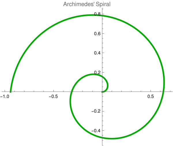
The Archimedean spiral (also known as Archimedes' spiral, the arithmetic spiral) is a spiral curve described in polar coordinates by the equation r = 𝑎 + bθ. In Cartesian coordinates (x, y), the parametric equations with respect to the parameter θ
(the angle of rotation in radians) are:
\[
x (\theta ) = \left( a + b\theta \right) \cos\theta , \qquad y (\theta ) = \left( a + b\theta \right) \sin\theta .
\]
An Archimedes' spiral appears on Jacob Bernoulli's tombstone due to a mason's mistake, as Bernoulli actually requested a logarithmic spiral because he viewed its self-similar properties as a metaphor for life after death and the Latin motto "Eadem mutata resurgo" ("Although changed, I shall arise the same").
(* Set parameters: starts at origin (a=0), turns expand by b=0.1 *)
a = 0;
b = 0.1;
ParametricPlot[
{(a + b*t) * Cos[t], (a + b*t) * Sin[t]},
{t, 0, 6 Pi}, (* 6 Pi gives exactly 3 full turns *)
PlotStyle -> Directive[Thick, Darker[Green]],
PlotLabel -> "Archimedes' Spiral",
Axes -> True
]
Figure 5.1: Archimedean spiral.
There are known some other spiral curves.
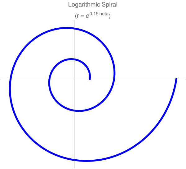
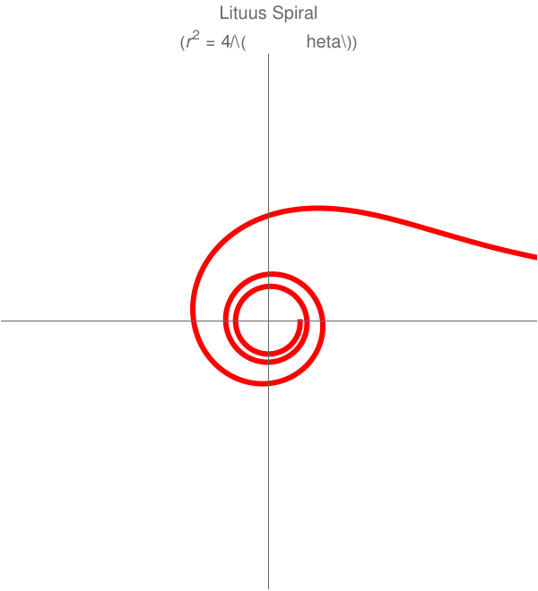
Logarithmic Spiral (Equiangular Spiral) expands exponentially, meaning its shape stays identical as it grows (self-similarity). The logarithmic spiral was first described by René Descartes in 1638. Its equation in polar is
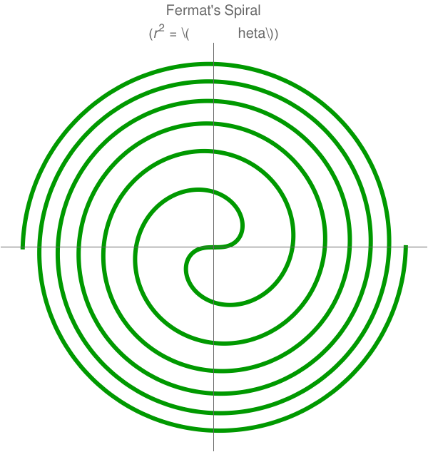
Fermat's Spiral (Parabolic Spiral) shares a close relationship with the Archimedean spiral but expands much more slowly because the radius depends on the square root of the angle.
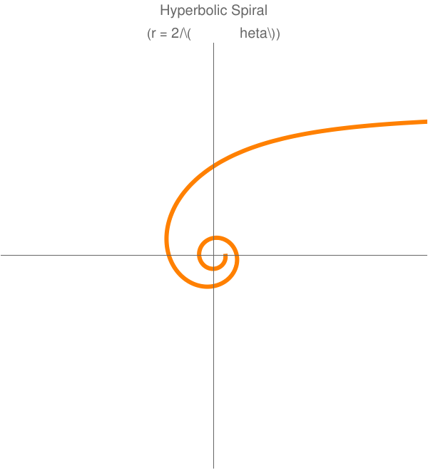
Hyperbolic Spiral (Reciprocal Spiral) acts as the inverse of an Archimedes' spiral. Instead of moving outward as the angle increases, it starts infinitely far away and winds inward toward the origin.
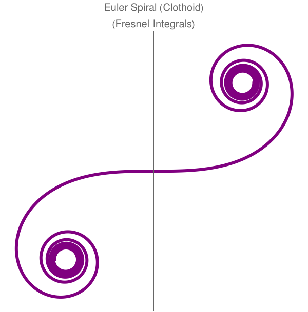
Clothoid (Euler Spiral / Cornu Spiral) is defined by a fundamental geometric property: its curvature increases linearly with its arc length.
This means as you travel along the curve, it turns tighter and tighter at a perfectly constant rate. The cleanest definition of the Euler spiral is given by its intrinsic equation, which relates its curvature (κ) directly to its arc length (s):
\[
\kappa = \frac{s}{a^2} .
\]
In Cartesian coordinates (x, y), we integrate the intrinsic property. This yields equations defined by the Fresnel Integrals:
\[
s (t) = a \int_0^t \,\cos \left( \frac{u^2}{2} \right) {\text d}u , \qquad y(t) = a \int_0^t \,\sin \left( \frac{u^2}{2} \right) {\text d}u .
\]
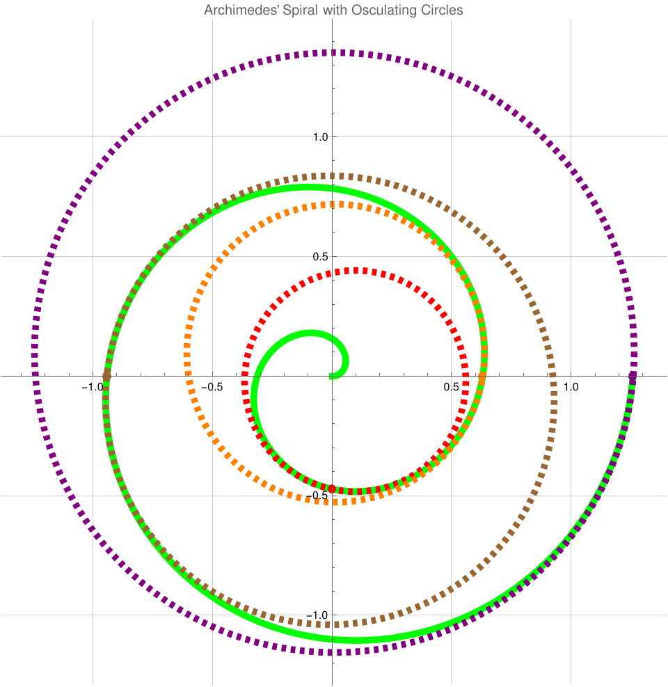
Now we plot the Archimedes' spiral along with the four osculating (touching) circles at the exact specified points. Every circle has the radius 1/κ(θ). The code automatically uses vector calculus to determine the exact radius of curvature and the center C coordinates for each circle.