Example 1: Let us consider a well known physical law, Newton's second law of motion: \[ m\,\frac{{\text d}^2 {\bf x}}{{\text d} y^2} = \mathbf{F} , \] where m is the mass of the object, x is its displacement vector in ℝ³, and F is acting force. To rewrite this law in non-dimensional form, let us assume that the characteristic values of mass #, length, and time in this equation are M, L, and T, respectively. The force term F in this equation has a dimension of (mass * Length/time²). Therefore, we define the following dimensionless quantities, \[ m^{\ast} = \frac{m}{M}, \quad {\bf x}^{\ast} = \frac{\bf x}{L} , \quad t^{\ast} = \frac{t}{T}, \quad {\bf F}^{\ast} = \frac{{\bf F}T^2}{ML} \] Then the left hand side of Newton's second law becomes \[ m\,\frac{{\text d}^2 {\bf x}}{{\text d} y^2} = Mm^{\ast} \frac{{\text d}^2 \left( L\mathbf{x}^{\ast} \right)}{{\text d}\left( T^2 t^{{\ast}2} \right)} = \frac{ML}{T^2} \,m^{\ast} \frac{{\text d}^2 \mathbf{x}^{\ast}}{{\text d} t^{{\ast}2}} . \] t the same time the right hand side of Newton's second law yields \[ \mathbf{F} = \frac{ML}{T^2}\,\mathbf{F}^{\ast} . \] Therefore, we can rewrite Newton's second law in new variables as \[ m^{\ast} \frac{{\text d}^2 \mathbf{x}^{\ast}}{{\text d} r^{{\ast}2}} = \mathbf{F}^{\ast}. \] This equation is independent of the physical units.    ■

Example 2: Let us consider the following modification of previous equation discussed in the previous example \[ m\,\frac{{\text d}^2 {\bf x}}{{\text d} y^2} = \mathbf{F} + \alpha \left( \frac{{\text d}{\bf x}}{{\text d}t} \right)^2 . \tag{2.1} \] The question naturally arises as to the impact of the additional term on the solution. Is it “small” or “large” compared to the other terms of the equation? To answer this question, we introduce the same non-dimensional quantities as in Example 1, and the additional term in Equation (2.1) becomes \[ \left( \frac{{\text d}{\bf x}}{{\text d}t} \right)^2 = \left( \frac{{\text d}\left( L\mathbf{x}^{\ast| \right)}{{\text d}\left( T t^{{\ast}} \right)} \right)^2 = \frac{L^2}{T^2} \left( \frac{{\text d}\mathbf{x}^{\ast}}{{\text d}t^{\ast}} \right)^2 . \] Therefore, Equation (2.1) leads to \[ \frac{ML}{T^2}\,m^{\ast} \frac{{\text d}^2 \mathbf{x}^{\ast}}{{\text d} t^{{\ast}2}} = \frac{ML}{T^2}\,\mathbf{F}^{\ast} + \alpha \frac{L^2}{T^2} \left( \frac{{\text d}\mathbf{x}^{\ast}}{{\text d}t^{\ast}} \right)^2 . \] Hence, \[ m^{\ast} \frac{{\text d}^2 \mathbf{x}^{\ast}}{{\text d} t^{{\ast}2}} = \mathbf{F}^{\ast} + \frac{aL}{M} \left( \frac{{\text d}\mathbf{x}^{\ast}}{{\text d}t^{\ast}} \right)^2 . \] It follows then that the size of the additional term in Equation (2.1) (as compared to other terms in this equation) is not determined by α alone but by the ratio α^✶ = αL/M. If α^✶ ≪ 1, we can treat the additional term in Equation (2.1) as a small perturbation. On the other hand if α^✶ ≈ 1, such a treatment will be inappropriate.

Another way to look on this issue is to realize that α is not a dimensionless number since each of the terms in Equation (2.1) must have the same dimension. Therefore α must have the dimension of (mass/length). Hence, the dimensionless form of this constant is (αL/M).    ■

Example 3: Let us consider the differential equation \[ \frac{{\text d}y}{{\text d}x} = 1 + a\, y^2 , \qquad \mbox{with} \quad a = 1 + \varepsilon , \tag{3.1} \] subject to the homogeneous initial condition \[ y(0) = 0 . \] This initial value problem also asks how smoothly its solution depends on variation of input coefficient 𝑎 near 𝑎 = 1 (this value is chosen for pedagogical reasons). Since the given differential equation is separable, we split it by dividing both sides by 1 + 𝑎y². This yields \[ \frac{{\text d}y}{1 + a\,y^2} = {\text d} x \qquad \Longrightarrow \qquad \int_0^y \frac{{\text d}y}{1 + a\,y^2} = x. \] Using Mathematica we find its solution to be \[ \mbox{arctan} \left( \sqrt{a}\,x \right) = x\,\sqrt{a} . \] Application of tangen to both sides gives \[ y (x, a) = \frac{1}{\sqrt{a}} \, \tan \left( x\,\sqrt{a} \right) , \qquad a = 1 + \varepsilon . %y( x, \varepsilon ) = \left( 1 + \varepsilon \right)^{-1/2} \tan \left[ \left( 1 + \varepsilon \right)^{1/2} x \right] . \] When ε = 0, the unperturbed solution become y₀ = tan(x). A Maclaurin series expansion of perturbed solution in ε is \[ y( x, \varepsilon ) = \tan x + \varepsilon \left( \frac{x}{2}\,\sec^2 x - \frac{1}{2}\,\tan x \right) + \cdots . \] Forgetting the exact solution for the moment, we assume that \[ y(x, \varepsilon ) = y^{(0)} (x) + \varepsilon \,y^((1)) + \cdots . \] Upon substitution this series into Eq.(3.1), we find \[ \frac{{\text d} y^{(0)}}{{\text d}x} + \varepsilon\,\frac{{\text d} y^{(1)}}{{\text d}x} + \cdots = 1 + \left( 1 + \varepsilon \right) \left[ \left( y^{(0)} \right)^2 + 2\varepsilon \,y^{(0)} y^{(1)} + \cdots \right] , \] so that \[ \frac{{\text d} y^{(1)}}{{\text d}x} = \left( y^{(0)} \right)^2 + 2 \,y^{(0)} y^{(1)} \] It is frequently the case, as here, that direct substitution provides the desired perturbation equation more easily than substitution into a general form. Rearranging the differential equation for y⁽¹⁾ into standard form and using the fact that y⁽⁰⁾(x) = tan(x), we obtain \[ \frac{{\text d} y^{(1)}}{{\text d}x} - 2\,y^{(1)} \tan x = \tan^2 x . \tag{3.2} \] An integrating factor for this equation satisfies \[ \frac{{\text d}\mu}{{\text d}x} + 2\mu\,\tan x = 0\qquad \Longrightarrow \qquad \frac{{\text d}\mu}{\mu} = -2\tanx \,{\text d}x . \] Multiplying both sides of Eq.(3.2) by \[ \mu (x) = \exp \left\{ -2 \int \tan x\,{\text d}x \right\} = \cos^2 x , \] we obtain an exact equation \[ \frac{\text d}{{\text d}x} \left[ y^{(1)} \cos^2 x \right] = \cos^2 x\,\tan^2 x = \sin^2 x . \] This allows us to determine y⁽¹⁾ explicitly. \[ y^{(1)} \cos^2 x = \frac{x}{2} - \frac{1}{4}\, \sin (2x) \quad \Longrightarrow \quad y^{(1)} = \frac{x}{2\cos^2 x} - \frac{\sin x}{2\,\cos x} . \]    ■

Example 3A: We atark the same problem \[ \frac{{\text d}y}{{\text d}x} = 1 + \left( 1 + \varepsilon \right) y^2 , \qquad y(0) = 0 , \tag{3.1} \] using the Adomian decomposition method (ADM for short). Application of this method does not depend on whether parameter ε is small or not. The value of this parameter affects the region of convergence \[ y = y(x, \varepsilon) = \sum_{n\ge 0} u_n (x) . \tag{3.2} \] The initial term is determined by solving the IVP: \[ \frac{{\text d} u_0}{{\text d}x} = 1 , \qquad u_0 (0) = 0 . \] Since this problem has a unique solution u₀ = x, we proceed with finding other terms. The non-linear term in Eq.(3.1) is decomposed to the series over Adomian polynomials: \[ f(y) = \left( 1 + \varepsilon \right) y^2 = \sum_{n\ge 0} A_n \left( u_0 , \ldots , u_n \right) , \tag{3.3} \] where \[ A_n = \frac{1}{n!} \, \frac{{\text d}^n}{{\text d}\lambda^n} \left[ f \left( \sum_{k\ge 0} u_k \lambda^k \right) \right]_{\lambda =0} , \quad n=0,1,2,\ldots . \] The first few Adomian polynomials for out non-linear function f(y) are \begin{align*} A_0 &= \left( 1 + \varepsilon \right) x^2 , \\ A_1 &= 2\left( 1 + \varepsilon \right) x\, u_1 , \\ A_2 &= \left( 1 + \varepsilon \right) u_1^2 +2 \left( 1 + \varepsilon \right) x\, u_2 , \\ A_3 &= 2 \left( 1 + \varepsilon \right) u_1 u_2 + 2 \left( 1 + \varepsilon \right) x\,u_3 . \end{align*} Each component in Eq.(3.2) is a unique solution of the initial value problem: \[ \frac{\text d}{{\text d}x}\, u_n = A_{n-1} , \qquad u_n (0) = 0, \quad n=1, 2, 3, \ldots . \] For n = 1, we have \[ \frac{\text d}{{\text d}x}\, u_1 =\left( 1 + \varepsilon \right) x^2 \qquad \Longrightarrow \qquad u_1 = \frac{x^3}{3} \left( 1 + \varepsilon \right) . \] For n = 2, we get \[ \frac{\text d}{{\text d}x}\, u_2 = \frac{2}{3} \left( 1 + \varepsilon \right)^2 x^4 \qquad \Longrightarrow \qquad u_2 = \frac{2 x^5}{15} \left( 1 + \varepsilon \right)^2 . \] Therefore, keeping these few terms, we obtain the ADM approximation \[ y (x, \varepsilon ) = x + \frac{x^3}{3} \left( 1 + \varepsilon \right) + \frac{2 x^5}{15} \left( 1 + \varepsilon \right)^2 + \cdots . \]    ■

Example 4: We consider a simple mathematical model describing oscillations of pendulum. Its bob is assumed to have mass m and length ℓ.

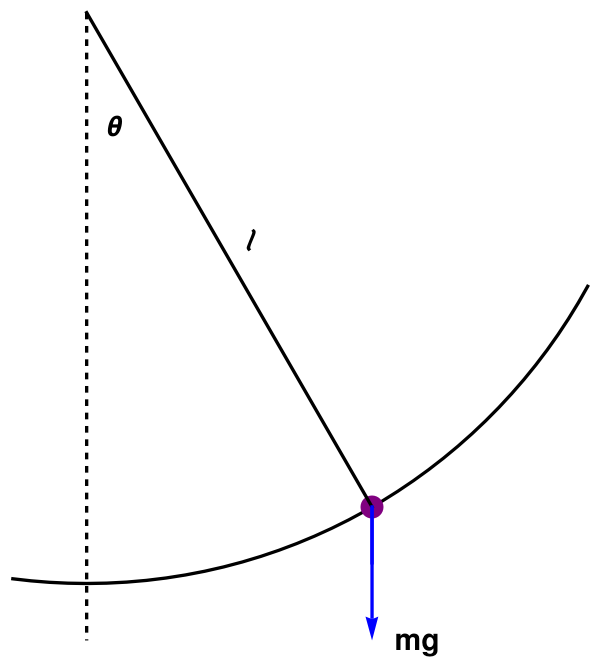
We consider an approximation that lead to derivation of so called simple pendulum model. Let denote by θ(t) the inclination of the rod to the vertical at time t. If s(t) denoted the distance the bob has moved from the vertical in a counterclockwise direction, then θℓ = s. Equating m(d²s/dt²) to the force component that is tangential to the path of the bob has moved, we obtain the following equation of motion: \[ m\ell\,\ddot{\theta} = -mg\,\sin\theta , \] where g is the acceleration due to gravity. The tension along the spring/rod does not enter because it acts normally to the path of the bob.

The equation of motion is convenient to write in the standard (when leading coefficient is 1) form: \[ \ddot{\theta} + \omega_0^2\sin\theta = 0, \qquad \omega_0 = \left( \frac{g}{\ell} \right)^{1/2} . \tag{4.1} \] Its motion is subject to the initial conditions: \[ \theta (0) = a , \qquad \dot{\theta}(0) = \Omega . \tag{4.2} \] Equations (4.2) and (4.2) comprise the initial value problem for simple pendulum motion.

Standard treatment of problem (4.1), (4.2) by perturbation method starts with linear approximation \[ \ddot{\theta} + \omega_0^2 \theta = 0 , \qquad \theta (0) = a, \quad \dot{\theta)(0) = \Omega . \] Its solution is given by

\[ \theta (t) = a\,\cos\left( \omega_0 t \right) + \frac{\Omega}{\omega_0} \,\sin \left( \omega_0 t \right) . \tag{4.3} \] An obvious inference from the solution is that, irrespective of the initial conditions, the motion is periodic with period \[ p_0 = \frac{2\pi}{\omega_0} = 2\pi \left( \frac{g}{\ell} \right)^{1/2} . \tag{4.4} \] This approximation is not adequate, however, if we interested in following motion of the mass point over many periods, for instance, the period given by (4.4) is not exactly right. According to the 'exact' equation (4.1), the motion is indeed periodic, but the correct period is \[ p = p_0 \,\frac{2}{\pi} \int_0^{\pi /2} \left( 1 - k^2 \sin^2 \psi \right)^{-1/2} {\text d} \psi , \] where k² = sin²(θ_m/2) and θ_m is the amplitude of the oscillation (i.e., the maximum value of |θ(t)}): \[ \theta_m = \max \left\vert \theta (t) \right\vert . \] With every swing of the pendulum, the approximate solution misestimates the time of maximum amplitude by a further increment of p − p₀. The error in period is about 0.2 percent for amplitude θ_m = π/18 radians. Thus, the solution to the approximate linear equation can be expected to be nearly the same as the solution to Eq.(4.1) only for a number of periods N such that N(p − p₀) is small compared to p.

To improve on the approximation, one might write Eq.(4.1) in the form \[ \ddot{\theta} + \omega_0^2 \theta = \omega_0^2 \left( \theta - \sin\theta \right) \] and then obtain a reasonable accurate value of the right-hand side by using the first approximation θ₀ of linear equation (4.3), namely, \[ \omega_0^2 \left( \theta - \sin\theta \right) = \omega_0^2 \left( \theta - \theta + \frac{\theta^3}{3!} - \frac{\theta^5}{5!} + \cdots \right) = \omega_0^2 \frac{\theta^3}{3!} - \cdots , \] is of the order of θ³, while the left-hand side is of the order θ. Thus, the smaller right-hand side can be ignored altogether to obtain an initial approximation θ₀(t). A better approximation should be obtained if substitution θ = θ₀ is made on the right-hand side, etc. Hence, the first attempt at an improved approximation θ₁(t) might be expected to satisfy \[ \ddot{\theta}_1 + \omega_0^2 \theta_1 = \omega_0^2 \left( \theta_0 - \sin\theta_0 \right), \qquad \theta_1 (0) = a , \quad \dot{\theta}_1 (0) = \Omega . \tag{4.5} \] However, an exact evaluation of the right-hand side (4.5) is almost impossible for θ₀. Instead, we replace Eq.(4.5) with the following approximation \[ \ddot{\theta}_1 + \omega_0^2 \theta_1 = \omega_0^2 \, \frac{\theta_0^3}{3!} , \qquad \theta_1 (0) = a , \quad \dot{\theta}_1 (0) = \Omega . \tag{4.6} \] In principle, repetition of the process will provide successively more accurate approximations. Therefore, this method is known as iteration (Latin iterare to do again), or successive approximations.    ■

Example 4A: Perturbation series approach is more convenient to apply for a new dependent variable \[ \Theta (t) = \frac{\theta (t)}{\theta_m} , \] where θ_m is the maximum amplitude: \[ \theta_m = \max_t \left\vert \theta (t) \right\vert . \] Intuitively, θ_m seems to provide a natural standard of comparison for the angular displacement. The new variable Θ satisfies |Θ| ≤ 1, and this proves usefulness in estimating the size of various terms.

Then the governing equation of motion becomes \[ \ddot{\Theta} + \omega_0^2 \Theta = \omega_0^2 \left( \Theta - \theta^{-1}_m \sin \theta_m \Theta \right) = \omega_0^2 \theta_m^2 \frac{\Theta^3}{6} + \cdots . \] Note that its right-hand side is of order (θ_m)² because |Θ| ≤ 1 and therefore it is very small compared to unity.

For simplicity, let us assume that the pendulum is released from rest, so Ω = 0. It is physically clear that θ_m = 𝑎, so our problem becomes \begin{align*} \ddot{\Theta} + \omega_0^2 \Theta &= \omega_0^2 \left( ]Theta - a^{-1} \sin a\Theta \right) \\ &= \omega_0^2 \sum_{n\ge 1} (-1)^{n+1} a^{2n} \frac{\Theta^{2n+1}}{(2n+1)!} , \\ &\quad \Theta (0) = 1, \quad \dot{\Theta}(0) = 0 . \end{align*} We seeks solution of this initial value problem in the following form: \[ \Theta = \Theta (t, a) = \Theta^{(0)} (t) _ a\, \Theta^{(1)} (t) + a^2 \Theta^{(2)} (t) + \cdots \tag{4A.1} \] Upon substitution this series into the differential equation, we obtain a sequence of equations subject to the following initial conditions \begin{align*} \Theta^{(0)} (0) &= 1 , \quad \dot{\Theta}^{(0)} (0) = 0 , \\ \Theta^{(n)} (0) &= 1 , \quad \dot{\Theta}^{(n)} (0) = 0 , \quad \mbox{for} \quad n\ge 1 . \end{align*} In this formulation, the dependence of the solution on amplitude 𝑎 is explicitly demonstrated. Note that if all the higher powers of the amplitude are neglected, we get the usual simple harmonic motion.

To ensure that our method works, one may try to prove convergence of series (4A.1). However, this turns out to be incorrect neither for necessary statement nor foe sufficient one. Even when such series is divergent, it can still be useful as an asymptotic series. On the other hand, convergence does not assure its usefulness. An inordinately large number of terms might have to be summed to obtain reasonable accuracy.

As a matter of fact, it can be shown that series (4A.1) is in general convergent in any finite interval 0 ≤ t ≤ T, provided that 𝑎 is sufficiently small (it follows from analytic dependence of the right-hand side of the differential equation). However, this does not assure usefulness of the solution for many periods, Upon carrying out calculations, one can show that \[ \Theta^{(0)} (t) = \cos\omega_0 t , \qquad \Theta^{(1)} (t) \equiv 0. \] Hence, the next approximation satisfies \[ \ddot{\Theta}^{(2)} + \omega_0^2 \Theta^{(2)} = \frac{\omega_0^2}{6} \,\cos^3 \omega_0 t. \] Using trigonometric identities (or computer algebra system), this equation can be shown to be equivalent to \[ \ddot{\Theta}^{(2)} + \omega_0^2 \Theta^{(2)} = \frac{\omega_0^2}{24} \left( \cos 3 \omega_0 t + 3\,\cos\omega_0 t \right) . \] This is a linear constant coefficient differential equation whose right-hand side contains a "resonant" term cos(ω₀t. Therefore, its solution contains a factor of t: \[ \Theta (t) = \frac{\sin \omega_0 t}{96} \left[ \sin (2\omega_0 t) + 6\,\omega_0 t \right] . \]

Note that product of two sine functions leads to appearance of more rapidly osci;;ating "higher harmonics," which is a typical feature of nonlinear phenomenon.

However, the term proportional to tsin(ω₀t) holds the center of our interest because it is not uniformly small for all time. Hence, approximation Θ⁽⁰⁾ + 𝑎²Θ⁽²⁾ is an improvement over Θ⁽⁰⁾ only for the time interval that Θ⁽⁰⁾ itself offers a reasonable approximation.    ■

Example 4P:

The Poincaré representation of solution Θ(t, 𝑎) is \begin{align*} \Theta &= \Theta^{(0)} (\tau ) + a \, \Theta^{(1)} (\tau ) + a^2 \Theta^{(2)} (\tau ) + \cdots , \tag{4P.1} \\ t &= \tau + a\,t^{(1)} (\tau ) + a^2 t^{(2)} (\tau ) + \cdots , \end{align*} where τ is a parameter. Poincaré's idea was to let solution Θ⁽⁰⁾(τ) take on the simple form (4P.1) in variable τ, but to distort the time scale so that the defects in the solution are removed. We expect to eliminate all secular (seculum means "generation" or "age" in Latin; hence, the word "secular" applies to processes of slow change) terms and to get the correct period with good approximation. The calculations are fairly complicated but can be simplified by noting that series (4P.1) should be in 𝑎².It also turns out that one may take all the correction terms to be a constant multiple of τ, thus, \[ t = \tau \left( 1 + a^2 h_2 \right) , \qquad h2 \mbox{ is a constant}. \] The equation for Θ⁽²⁾ is then found to be \[ \left( \frac{{\text d}^2}{{\text d}\tau^2} + \omega_0^2 \right) \Theta^{(2)} = 2h_2 \frac{{\text d}^2}{{\text d}\tau^2} \,\Theta^{(0)} + \frac{\omega_0^2}{24} \left( \cos 3\omega_0 \tau + 3\,\cos \omega_0 \tau \right) . \] Using exact solution for Θ⁽⁰⁾, the expression above can be reduced to \[ \left( \frac{{\text d}^2}{{\text d}\tau^2} + \omega_0^2 \right) \Theta^{(2)} = \omega_0^2 \left( \frac{1}{8} - 2 h_2 \right) \cos\omega_0\tau + \frac{\omega_0^2}{24}\,\cos 3\omega_0 \tau . \] Although the cosω₀τ term on the right-hand side would lead to an undesirable secular term proportional to τ sinω₀τ, it can be avoided by taking \[ h_2 = \frac{1}{16} . \] The period in &tau becomes 2π/ω₀ to this approximation, but is (2π/ω₀)(1 + 𝑎²h₂) in t.

   ■

1. Upon multiplication of the pendulum equation by derivative \( \displaystyle \quad \dot{\theta} , \quad \) show that its first integral is \[ \frac{1}{2} \left( \dot{\theta} \right)^2 = \omega_0^2 \left( \cos\theta - \cos a \right) = 2 \omega_0^2 \left( \sin^2 \frac{a}{2} - \sin^2 \frac{\theta}{2} \right) , \] where 𝑎 is the maximum amplitude. Verify that further transformation \[ \sin\frac{\theta}{2} = \sin\frac{a}{2}\,\sin\psi \] brings the solution into the form \[ t = -\frac{1}{\omega_0} \int_{\pi /2}^{\psi} \left( 1 - k^2 \sin^2 \psi \right)^{-1/2} {\text d}\psi , \qquad \theta (0) = a , \] where \( \displaystyle \quad k^2 = \sin^2 \frac{a}{2} . \)

2. Hadamard, Jacques (1902). Sur les problèmes aux dérivées partielles et leur signification physique. Princeton University Bulletin. pp. 49–52.
4. Tikhonov, A. N.; Arsenin, V. Y. (1977). Solutions of ill-Posed Problems. New York: Winston. ISBN 0-470-99124-0.